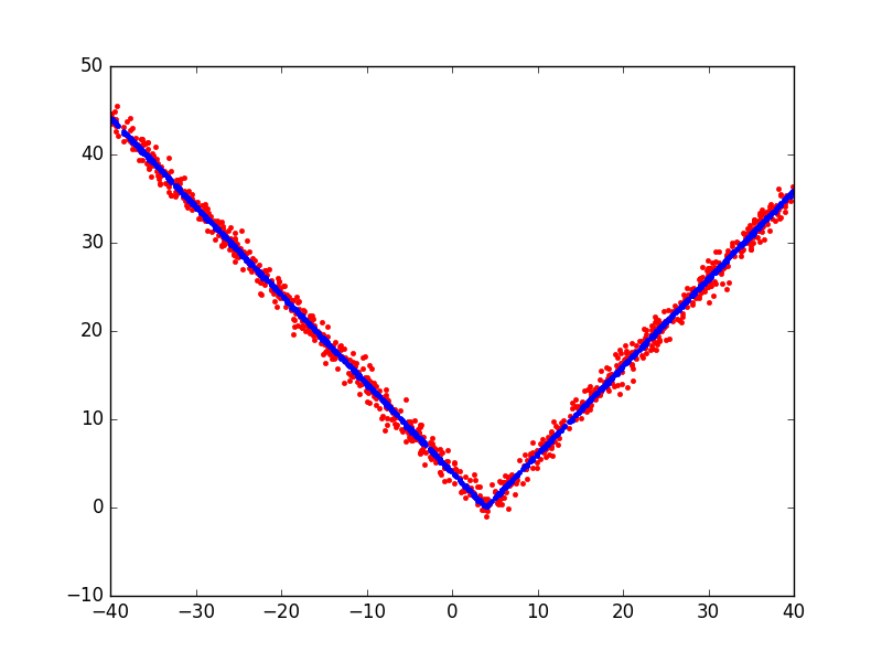
Plotting the absolute value function
A simple example plotting a fit of the absolute value function.
Out:
  Beginning forward pass
-------------------------------------------------------------------
iter  parent  var  knot  mse         terms  gcv      rsq    grsq
-------------------------------------------------------------------
0     -       -    -     135.278633  1      135.550  0.000  0.000
1     0       6    537   0.928785  3      0.940  0.993  0.993
2     0       0    377   0.918642  5      0.939  0.993  0.993
---------------------------------------------------------------
Stopping Condition 2: Improvement below threshold
Beginning pruning pass
--------------------------------------------
iter  bf  terms  mse   gcv    rsq    grsq
--------------------------------------------
0     -   5      0.92  0.939  0.993  0.993
1     4   4      0.92  0.939  0.993  0.993
2     3   3      0.93  0.940  0.993  0.993
3     1   2      83.82  84.410  0.380  0.377
4     2   1      135.28  135.550  0.000  0.000
------------------------------------------------
Selected iteration: 1
Forward Pass
-------------------------------------------------------------------
iter  parent  var  knot  mse         terms  gcv      rsq    grsq
-------------------------------------------------------------------
0     -       -    -     135.278633  1      135.550  0.000  0.000
1     0       6    537   0.928785    3      0.940    0.993  0.993
2     0       0    377   0.918642    5      0.939    0.993  0.993
-------------------------------------------------------------------
Stopping Condition 2: Improvement below threshold

Pruning Pass
------------------------------------------------
iter  bf  terms  mse     gcv      rsq    grsq
------------------------------------------------
0     -   5      0.92    0.939    0.993  0.993
1     4   4      0.92    0.939    0.993  0.993
2     3   3      0.93    0.940    0.993  0.993
3     1   2      83.82   84.410   0.380  0.377
4     2   1      135.28  135.550  0.000  0.000
------------------------------------------------
Selected iteration: 1

Earth Model
-------------------------------------
Basis Function  Pruned  Coefficient
-------------------------------------
(Intercept)     No      0.0693416
h(x6-3.93775)   No      0.995325
h(3.93775-x6)   No      1.00427
h(x0-13.1076)   No      -0.00984883
h(13.1076-x0)   Yes     None
-------------------------------------
MSE: 0.9230, GCV: 0.9389, RSQ: 0.9932, GRSQ: 0.9931
import numpy
import matplotlib.pyplot as plt
from pyearth import Earth

# Create some fake data
numpy.random.seed(2)
m = 1000
n = 10
X = 80 * numpy.random.uniform(size=(m, n)) - 40
y = numpy.abs(X[:, 6] - 4.0) + 1 * numpy.random.normal(size=m)

# Fit an Earth model
model = Earth(max_degree=1, verbose=True)
model.fit(X, y)

# Print the model
print(model.trace())
print(model.summary())

# Plot the model
y_hat = model.predict(X)
plt.figure()
plt.plot(X[:, 6], y, 'r.')
plt.plot(X[:, 6], y_hat, 'b.')
plt.show()
Total running time of the script: (0 minutes 0.165 seconds)
Download Python source code:
plot_v_function.py
Download IPython notebook:
plot_v_function.ipynb