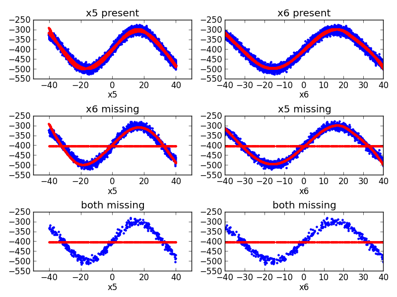
Plotting sine function with redundant predictors an missing data
An example plotting a fit of the sine function. There are two redundant predictors, each of which has independent and random missingness.
Out:
  Beginning forward pass
---------------------------------------------------------------------
iter  parent  var  knot  mse          terms  gcv       rsq    grsq
---------------------------------------------------------------------
0     -       -    -     4399.475105  1      4400.355  0.000  0.000
1     0       6    484   3218.482202  5      3225.575  0.268  0.267
2     3       6    7115  1000.371913  7      1003.581  0.773  0.772
3     0       5    1997  864.281682  11     868.794  0.804  0.803
4     10      5    584   587.091344  13     590.748  0.867  0.866
5     3       5    2524  366.234325  17     369.256  0.917  0.916
6     10      6    7684  282.087284  21     284.987  0.936  0.935
7     5       6    4061  278.832597  23     281.982  0.937  0.936
-------------------------------------------------------------------
Stopping Condition 2: Improvement below threshold
Beginning pruning pass
------------------------------------------------
iter  bf  terms  mse     gcv      rsq    grsq
------------------------------------------------
0     -   23     278.84  281.989  0.937  0.936
1     8   22     278.84  281.848  0.937  0.936
2     13  21     278.84  281.706  0.937  0.936
3     1   20     278.84  281.565  0.937  0.936
4     17  19     278.84  281.423  0.937  0.936
5     19  18     278.85  281.292  0.937  0.936
6     21  17     278.92  281.220  0.937  0.936
7     16  16     279.59  281.753  0.936  0.936
8     22  15     284.83  286.895  0.935  0.935
9     3   14     315.12  317.240  0.928  0.928
10    2   13     397.83  400.308  0.910  0.909
11    18  12     533.09  536.137  0.879  0.878
12    20  11     572.89  575.885  0.870  0.869
13    4   10     637.45  640.460  0.855  0.854
14    6   9      793.57  796.916  0.820  0.819
15    15  8      897.20  900.533  0.796  0.795
16    5   7      934.71  937.707  0.788  0.787
17    14  6      1017.38  1020.134  0.769  0.768
18    11  5      1258.44  1261.214  0.714  0.713
19    7   4      2635.44  2639.922  0.401  0.400
20    9   3      3192.33  3196.161  0.274  0.274
21    12  2      4039.23  4042.060  0.082  0.081
22    10  1      4399.48  4400.355  -0.000  -0.000
----------------------------------------------------
Selected iteration: 6
Earth Model
-----------------------------------------------------------------------------------------------------------------------------------------------
Basis Function                                                                                                            Pruned  Coefficient
-----------------------------------------------------------------------------------------------------------------------------------------------
(Intercept)                                                                                                               No      -477.431
present(x6)                                                                                                               Yes     None
missing(x6)                                                                                                               No      72.659
C(x6|s=+1,-32.2065,-24.4145,-7.42951)*present(x6)                                                                         No      1.7703
C(x6|s=-1,-32.2065,-24.4145,-7.42951)*present(x6)                                                                         No      10.543
C(x6|s=+1,-7.42951,9.55548,21.7265)*C(x6|s=+1,-32.2065,-24.4145,-7.42951)*present(x6)                                     No      -0.232449
C(x6|s=-1,-7.42951,9.55548,21.7265)*C(x6|s=+1,-32.2065,-24.4145,-7.42951)*present(x6)                                     No      -0.35568
present(x5)                                                                                                               No      113.492
missing(x5)                                                                                                               Yes     None
C(x5|s=+1,5.38057,22.2377,31.1865)*present(x5)                                                                            No      -11.1024
C(x5|s=-1,5.38057,22.2377,31.1865)*present(x5)                                                                            No      -2.39991
C(x5|s=+1,-25.8212,-11.4766,5.38057)*C(x5|s=-1,5.38057,22.2377,31.1865)*present(x5)                                       No      0.222427
C(x5|s=-1,-25.8212,-11.4766,5.38057)*C(x5|s=-1,5.38057,22.2377,31.1865)*present(x5)                                       No      0.260225
present(x5)*C(x6|s=+1,-32.2065,-24.4145,-7.42951)*present(x6)                                                             Yes     None
missing(x5)*C(x6|s=+1,-32.2065,-24.4145,-7.42951)*present(x6)                                                             No      4.96007
C(x5|s=+1,-15.4729,9.21999,24.6777)*present(x5)*C(x6|s=+1,-32.2065,-24.4145,-7.42951)*present(x6)                         No      0.210823
C(x5|s=-1,-15.4729,9.21999,24.6777)*present(x5)*C(x6|s=+1,-32.2065,-24.4145,-7.42951)*present(x6)                         No      0.00366201
present(x6)*C(x5|s=-1,5.38057,22.2377,31.1865)*present(x5)                                                                Yes     None
missing(x6)*C(x5|s=-1,5.38057,22.2377,31.1865)*present(x5)                                                                No      -5.024
C(x6|s=+1,-25.7228,-11.4472,14.2662)*present(x6)*C(x5|s=-1,5.38057,22.2377,31.1865)*present(x5)                           Yes     None
C(x6|s=-1,-25.7228,-11.4472,14.2662)*present(x6)*C(x5|s=-1,5.38057,22.2377,31.1865)*present(x5)                           No      -0.24299
C(x6|s=+1,21.7265,33.8976,36.9386)*C(x6|s=+1,-7.42951,9.55548,21.7265)*C(x6|s=+1,-32.2065,-24.4145,-7.42951)*present(x6)  Yes     None
C(x6|s=-1,21.7265,33.8976,36.9386)*C(x6|s=+1,-7.42951,9.55548,21.7265)*C(x6|s=+1,-32.2065,-24.4145,-7.42951)*present(x6)  No      -0.00262933
-----------------------------------------------------------------------------------------------------------------------------------------------
MSE: 279.9548, GCV: 282.2646, RSQ: 0.9364, GRSQ: 0.9359
import numpy
import matplotlib.pyplot as plt

from pyearth import Earth

# Create some fake data
numpy.random.seed(2)
m = 10000
n = 10
X = 80 * numpy.random.uniform(size=(m, n)) - 40
X[:, 5] = X[:, 6] + numpy.random.normal(0, .1, m)
y = 100 * \
    (numpy.sin((X[:, 5] + X[:, 6]) / 20) - 4.0) + \
    10 * numpy.random.normal(size=m)
missing = numpy.random.binomial(1, .2, (m, n)).astype(bool)
X_full = X.copy()
X[missing] = None
idx5 = (1 - missing[:, 5]).astype(bool)
idx6 = (1 - missing[:, 6]).astype(bool)

# Fit an Earth model
model = Earth(max_degree=5, minspan_alpha=.5, allow_missing=True,
              enable_pruning=True, thresh=.001, smooth=True, verbose=2)
model.fit(X, y)
# Print the model
print(model.summary())

# Plot the model
y_hat = model.predict(X)
fig = plt.figure()

ax1 = fig.add_subplot(3, 2, 1)
ax1.plot(X_full[idx5, 5], y[idx5], 'b.')
ax1.plot(X_full[idx5, 5], y_hat[idx5], 'r.')
ax1.set_xlim(-40, 40)
ax1.set_title('x5 present')
ax1.set_xlabel('x5')

ax2 = fig.add_subplot(3, 2, 2)
ax2.plot(X_full[idx6, 6], y[idx6], 'b.')
ax2.plot(X_full[idx6, 6], y_hat[idx6], 'r.')
ax2.set_xlim(-40, 40)
ax2.set_title('x6 present')
ax2.set_xlabel('x6')

ax3 = fig.add_subplot(3, 2, 3, sharex=ax1)
ax3.plot(X_full[~idx6, 5], y[~idx6], 'b.')
ax3.plot(X_full[~idx6, 5], y_hat[~idx6], 'r.')
ax3.set_title('x6 missing')
ax3.set_xlabel('x5')

ax4 = fig.add_subplot(3, 2, 4, sharex=ax2)
ax4.plot(X_full[~idx5, 6], y[~idx5], 'b.')
ax4.plot(X_full[~idx5, 6], y_hat[~idx5], 'r.')
ax4.set_title('x5 missing')
ax4.set_xlabel('x6')

ax5 = fig.add_subplot(3, 2, 5, sharex=ax1)
ax5.plot(X_full[(~idx6) & (~idx5), 5], y[(~idx6) & (~idx5)], 'b.')
ax5.plot(X_full[(~idx6) & (~idx5), 5], y_hat[(~idx6) & (~idx5)], 'r.')
ax5.set_title('both missing')
ax5.set_xlabel('x5')

ax6 = fig.add_subplot(3, 2, 6, sharex=ax2)
ax6.plot(X_full[(~idx6) & (~idx5), 6], y[(~idx6) & (~idx5)], 'b.')
ax6.plot(X_full[(~idx6) & (~idx5), 6], y_hat[(~idx6) & (~idx5)], 'r.')
ax6.set_title('both missing')
ax6.set_xlabel('x6')

fig.tight_layout()
plt.show()
Total running time of the script: (0 minutes 10.316 seconds)
Download Python source code:
plot_missing_data_problem.py
Download IPython notebook:
plot_missing_data_problem.ipynb