Cross-Validation for Generalized Linear Models

This example shows how to use cross-validation to automatically select the optimal regularization parameter for generalized linear models.

# Author: Florian Kozikowski

import numpy as np
import matplotlib.pyplot as plt

from skglm.utils.data import make_correlated_data
from skglm.cv import GeneralizedLinearEstimatorCV
from skglm.estimators import GeneralizedLinearEstimator
from skglm.datafits import Quadratic
from skglm.penalties import L1_plus_L2
from skglm.solvers import AndersonCD

Generate correlated data with sparse ground truth

X, y, true_coef = make_correlated_data(
    n_samples=150, n_features=300, random_state=42
)

Fit model using cross-validation

The CV estimator automatically finds the best regularization strength

estimator = GeneralizedLinearEstimatorCV(
    datafit=Quadratic(),
    penalty=L1_plus_L2(alpha=1.0, l1_ratio=0.5),
    solver=AndersonCD(max_iter=100),
    cv=5,
    n_alphas=50,
)
estimator.fit(X, y)

print(f"Best alpha: {estimator.alpha_:.3f}")
n_nonzero = np.sum(estimator.coef_ != 0)
n_true_nonzero = np.sum(true_coef != 0)
print(f"Non-zero coefficients: {n_nonzero} (true: {n_true_nonzero})")

Best alpha: 0.142
Non-zero coefficients: 94 (true: 60)

Visualize the cross-validation path

Plot shows how CV balances model complexity with prediction performance

# Get mean CV scores
mean_scores = np.mean(estimator.scores_path_, axis=1)
std_scores = np.std(estimator.scores_path_, axis=1)
best_idx = np.argmax(mean_scores)
best_alpha = estimator.alphas_[best_idx]

# Compute coefficient paths
coef_paths = []
for alpha in estimator.alphas_:
    est_temp = GeneralizedLinearEstimator(
        datafit=Quadratic(),
        penalty=L1_plus_L2(alpha=alpha, l1_ratio=0.5),
        solver=AndersonCD(max_iter=100)
    )
    est_temp.fit(X, y)
    coef_paths.append(est_temp.coef_)
coef_paths = np.array(coef_paths)

fig, (ax1, ax2) = plt.subplots(2, 1, figsize=(8, 10), sharex=True)

ax1.semilogx(estimator.alphas_, -mean_scores, 'b-', linewidth=2, label='MSE')
ax1.fill_between(estimator.alphas_,
                 -mean_scores - std_scores,
                 -mean_scores + std_scores,
                 alpha=0.2, label='±1 std. dev.')
ax1.axvline(best_alpha, color='red', linestyle='--',
            label=f'Best alpha = {best_alpha:.2e}')
ax1.set_ylabel('MSE')
ax1.set_title('Cross-Validation Score vs. Regularization')
ax1.legend(loc='best')
ax1.grid(True, alpha=0.3)
ax1.set_xlabel('alpha')

for j in range(coef_paths.shape[1]):
    ax2.semilogx(estimator.alphas_, coef_paths[:, j], lw=1, alpha=0.3)
ax2.axvline(best_alpha, color='red', linestyle='--')
ax2.set_xlabel('alpha')
ax2.set_ylabel('Coefficient value')
ax2.set_title('Regularization Path of Coefficients')
ax2.grid(True, alpha=0.3)

plt.tight_layout()
plt.show()

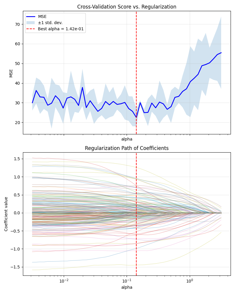
Top panel: Mean CV MSE shows U-shape, minimized at chosen alpha for optimal bias-variance tradeoff.

Bottom panel: At this alpha, most coefficients are shrunk (many near zero), highlighting a sparse subset of key predictors.

Visualize distance to true coefficients

Compute how well different regularization strengths recover the true coefficients

distances = []
for alpha in estimator.alphas_:
    est_temp = GeneralizedLinearEstimator(
        datafit=Quadratic(),
        penalty=L1_plus_L2(alpha=alpha, l1_ratio=0.5),
        solver=AndersonCD(max_iter=100)
    )
    est_temp.fit(X, y)
    distances.append(np.linalg.norm(est_temp.coef_ - true_coef, ord=1))

plt.figure(figsize=(8, 5))
plt.loglog(estimator.alphas_, distances, 'b-', linewidth=2)
plt.axvline(estimator.alpha_, color='red', linestyle='--',
            label=f'CV-selected alpha = {estimator.alpha_:.3f}')
plt.xlabel('Alpha (regularization strength)')
plt.ylabel('L1 distance to true coefficients')
plt.title('Recovery of True Coefficients')
plt.legend()
plt.grid(True, alpha=0.3)
plt.show()

print(
    f"Distance at CV-selected alpha: "
    f"{np.linalg.norm(estimator.coef_ - true_coef, ord=1):.3f}")

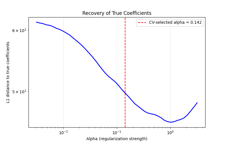
Distance at CV-selected alpha: 40.822

The U-shaped curve shows two failure modes: small alpha doesn’t induce enough sparsity (keeping noisy/irrelevant features), while large alpha overshrinks all coefficients including the true signals. Cross-validation finds a good balance without needing access to the ground truth.