Smooth Quantile Regression with QuantileHuber

This example compares sklearn’s standard quantile regression with skglm’s smooth approximation. Skglm’s quantile regression uses a smooth Huber-like approximation (quadratic near zero, linear in the tails) to replace the non-differentiable pinball loss. Progressive smoothing enables efficient gradient-based optimization, maintaining speed and accuracy also on large-scale, high-dimensional datasets.

# Author: Florian Kozikowski
import numpy as np
import time
import matplotlib.pyplot as plt

from sklearn.datasets import make_regression
from sklearn.linear_model import QuantileRegressor
from skglm.experimental.quantile_huber import QuantileHuber, SmoothQuantileRegressor

# Generate regression data
X, y = make_regression(n_samples=1000, n_features=10, noise=0.1, random_state=0)
tau = 0.8  # 80th percentile

Compare standard vs smooth quantile regression

Both methods solve the same problem but with different loss functions.

# Standard quantile regression (sklearn)
start = time.time()
sk_model = QuantileRegressor(quantile=tau, alpha=0.1)
sk_model.fit(X, y)
sk_time = time.time() - start

# Smooth quantile regression (skglm)
start = time.time()
smooth_model = SmoothQuantileRegressor(
    quantile=tau,
    alpha=0.1,
    delta_init=0.5,      # Initial smoothing parameter
    delta_final=0.01,    # Final smoothing (smaller = closer to true quantile)
    n_deltas=5           # Number of continuation steps
)
smooth_model.fit(X, y)
smooth_time = time.time() - start

Evaluate both methods

Coverage: fraction of true values below predictions (should ≈ tau) Pinball loss: standard quantile regression evaluation metric

Note: No robust benchmarking conducted yet. The speed advantagous likely only shows on large-scale, high-dimensional datasets. The sklearn implementation is likely faster on small datasets.

def pinball_loss(residuals, quantile):
    return np.mean(residuals * (quantile - (residuals < 0)))


sk_pred = sk_model.predict(X)
smooth_pred = smooth_model.predict(X)

print(f"{'Method':<15} {'Coverage':<10} {'Time (s)':<10} {'Pinball Loss':<12}")
print("-" * 50)
print(f"{'Sklearn':<15} {np.mean(y <= sk_pred):<10.3f} {sk_time:<10.3f} "
      f"{pinball_loss(y - sk_pred, tau):<12.4f}")
print(f"{'SmoothQuantile':<15} {np.mean(y <= smooth_pred):<10.3f} {smooth_time:<10.3f} "
      f"{pinball_loss(y - smooth_pred, tau):<12.4f}")

Method          Coverage   Time (s)   Pinball Loss
--------------------------------------------------
Sklearn         0.799      0.066      28.2682
SmoothQuantile  0.798      2.027      28.2699

Visualize the smooth approximation

The smooth loss approximates the pinball loss but with continuous gradients

fig, (ax1, ax2) = plt.subplots(1, 2, figsize=(10, 4))

# Show loss and gradient for different quantile levels
residuals = np.linspace(-3, 3, 500)
delta = 0.5
quantiles = [0.1, 0.5, 0.9]

for tau_val in quantiles:
    qh = QuantileHuber(quantile=tau_val, delta=delta)
    loss = [qh._loss_sample(r) for r in residuals]
    grad = [qh._grad_per_sample(r) for r in residuals]

    # Compute pinball loss for each residual
    pinball_loss = [r * (tau_val - (r < 0)) for r in residuals]

    # Plot smooth loss and pinball loss
    ax1.plot(residuals, loss, label=f"τ={tau_val}", linewidth=2)
    ax1.plot(residuals, pinball_loss, '--', alpha=0.4, color='gray',
             label=f"Pinball τ={tau_val}")
    ax2.plot(residuals, grad, label=f"τ={tau_val}", linewidth=2)

# Add vertical lines and shading showing delta boundaries
for ax in [ax1, ax2]:
    ax.axvline(-delta, color='gray', linestyle='--', alpha=0.7, linewidth=1.5)
    ax.axvline(delta, color='gray', linestyle='--', alpha=0.7, linewidth=1.5)
    # Add shading for quadratic region
    ax.axvspan(-delta, delta, alpha=0.15, color='gray')

# Add delta labels
ax1.text(-delta, 0.1, '−δ', ha='right', va='bottom', color='gray', fontsize=10)
ax1.text(delta, 0.1, '+δ', ha='left', va='bottom', color='gray', fontsize=10)

ax1.set_title(f"Smooth Quantile Loss (δ={delta})", fontsize=12)
ax1.set_xlabel("Residual")
ax1.set_ylabel("Loss")
ax1.legend(loc='upper left')
ax1.grid(True, alpha=0.3)

ax2.set_title("Gradient (continuous everywhere)", fontsize=12)
ax2.set_xlabel("Residual")
ax2.set_ylabel("Gradient")
ax2.legend(loc='upper left')
ax2.grid(True, alpha=0.3)

plt.tight_layout()
plt.show()

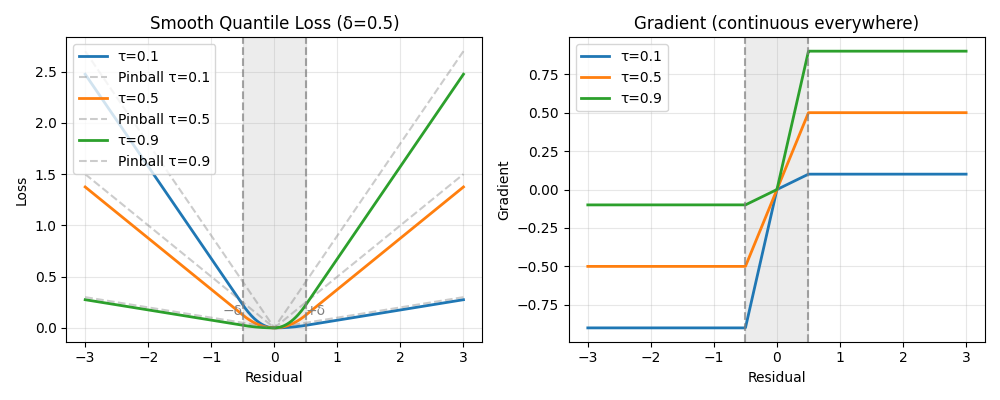
The left plot shows the asymmetric loss: tau=0.1 penalizes overestimation more, while tau=0.9 penalizes underestimation. As delta decreases towards zero, the loss function approaches the standard pinball loss. The right plot reveals the key advantage: gradients transition smoothly through zero, unlike standard quantile regression which has a kink. This smoothing enables fast convergence with gradient-based solvers.