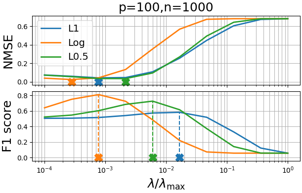
Regularization paths for the Graphical Lasso and its Adaptive variation

This example demonstrates how non-convex penalties in the Adaptive Graphical Lasso can achieve superior sparsity recovery compared to the standard L1 penalty.

The Adaptive Graphical Lasso uses iterative reweighting to approximate non-convex penalties, following Candès et al. (2007). Non-convex penalties often produce better sparsity patterns by more aggressively shrinking small coefficients while preserving large ones.

We compare three approaches:

• L1: Standard Graphical Lasso with L1 penalty

• Log: Adaptive approach with logarithmic penalty

• L0.5: Adaptive approach with L0.5 penalty

The plots show normalized mean square error (NMSE) for reconstruction accuracy and F1 score for sparsity pattern recovery across different regularization levels.

# Authors: Can Pouliquen
#          Mathurin Massias
#          Florian Kozikowski

import numpy as np
from numpy.linalg import norm
import matplotlib.pyplot as plt
from sklearn.metrics import f1_score

from skglm.covariance import GraphicalLasso, AdaptiveGraphicalLasso
from skglm.penalties.separable import LogSumPenalty, L0_5
from skglm.utils.data import make_dummy_covariance_data

Generate synthetic sparse precision matrix data

p = 100
n = 1000
S, _, Theta_true, alpha_max = make_dummy_covariance_data(n, p)
alphas = alpha_max*np.geomspace(1, 1e-4, num=10)

Setup models with different penalty functions

penalties = ["L1", "Log", "L0.5"]
n_reweights = 5  # Number of adaptive reweighting iterations
models_tol = 1e-4

models = [
    # Standard Graphical Lasso with L1 penalty
    GraphicalLasso(algo="primal", warm_start=True, tol=models_tol),

    # Adaptive Graphical Lasso with logarithmic penalty
    AdaptiveGraphicalLasso(warm_start=True,
                           penalty=LogSumPenalty(alpha=1.0, eps=1e-10),
                           n_reweights=n_reweights,
                           tol=models_tol),

    # Adaptive Graphical Lasso with L0.5 penalty
    AdaptiveGraphicalLasso(warm_start=True,
                           penalty=L0_5(alpha=1.0),
                           n_reweights=n_reweights,
                           tol=models_tol),
]

Compute regularization paths

nmse_results = {penalty: [] for penalty in penalties}
f1_results = {penalty: [] for penalty in penalties}


# Fit models across regularization path
for i, (penalty, model) in enumerate(zip(penalties, models)):
    print(f"Fitting {penalty} penalty across {len(alphas)} regularization values...")
    for alpha_idx, alpha in enumerate(alphas):
        print(
            f"  alpha {alpha_idx+1}/{len(alphas)}: "
            f"lambda/lambda_max = {alpha/alpha_max:.1e}",
            end="")

        model.alpha = alpha
        model.fit(S, mode='precomputed')

        Theta_est = model.precision_
        nmse = norm(Theta_est - Theta_true)**2 / norm(Theta_true)**2
        f1_val = f1_score(Theta_est.flatten() != 0., Theta_true.flatten() != 0.)

        nmse_results[penalty].append(nmse)
        f1_results[penalty].append(f1_val)

        print(f"NMSE: {nmse:.3f}, F1: {f1_val:.3f}")
    print(f"{penalty} penalty complete!\n")

Fitting L1 penalty across 10 regularization values...
  alpha 1/10: lambda/lambda_max = 1.0e+00NMSE: 0.682, F1: 0.058
  alpha 2/10: lambda/lambda_max = 3.6e-01NMSE: 0.674, F1: 0.123
  alpha 3/10: lambda/lambda_max = 1.3e-01NMSE: 0.606, F1: 0.330
  alpha 4/10: lambda/lambda_max = 4.6e-02NMSE: 0.447, F1: 0.519
  alpha 5/10: lambda/lambda_max = 1.7e-02NMSE: 0.255, F1: 0.582
  alpha 6/10: lambda/lambda_max = 6.0e-03NMSE: 0.108, F1: 0.573
  alpha 7/10: lambda/lambda_max = 2.2e-03NMSE: 0.046, F1: 0.541
  alpha 8/10: lambda/lambda_max = 7.7e-04NMSE: 0.042, F1: 0.516
  alpha 9/10: lambda/lambda_max = 2.8e-04NMSE: 0.059, F1: 0.507
  alpha 10/10: lambda/lambda_max = 1.0e-04NMSE: 0.073, F1: 0.505
L1 penalty complete!

Fitting Log penalty across 10 regularization values...
  alpha 1/10: lambda/lambda_max = 1.0e+00NMSE: 0.682, F1: 0.058
  alpha 2/10: lambda/lambda_max = 3.6e-01NMSE: 0.682, F1: 0.058
  alpha 3/10: lambda/lambda_max = 1.3e-01NMSE: 0.682, F1: 0.058
  alpha 4/10: lambda/lambda_max = 4.6e-02NMSE: 0.676, F1: 0.073
  alpha 5/10: lambda/lambda_max = 1.7e-02NMSE: 0.569, F1: 0.220
  alpha 6/10: lambda/lambda_max = 6.0e-03NMSE: 0.355, F1: 0.485
  alpha 7/10: lambda/lambda_max = 2.2e-03NMSE: 0.133, F1: 0.724
  alpha 8/10: lambda/lambda_max = 7.7e-04NMSE: 0.043, F1: 0.810
  alpha 9/10: lambda/lambda_max = 2.8e-04NMSE: 0.024, F1: 0.750
  alpha 10/10: lambda/lambda_max = 1.0e-04NMSE: 0.039, F1: 0.640
Log penalty complete!

Fitting L0.5 penalty across 10 regularization values...
  alpha 1/10: lambda/lambda_max = 1.0e+00NMSE: 0.682, F1: 0.058
  alpha 2/10: lambda/lambda_max = 3.6e-01NMSE: 0.682, F1: 0.059
  alpha 3/10: lambda/lambda_max = 1.3e-01NMSE: 0.644, F1: 0.142
  alpha 4/10: lambda/lambda_max = 4.6e-02NMSE: 0.494, F1: 0.373
  alpha 5/10: lambda/lambda_max = 1.7e-02NMSE: 0.270, F1: 0.615
  alpha 6/10: lambda/lambda_max = 6.0e-03NMSE: 0.095, F1: 0.726
  alpha 7/10: lambda/lambda_max = 2.2e-03NMSE: 0.034, F1: 0.685
  alpha 8/10: lambda/lambda_max = 7.7e-04NMSE: 0.035, F1: 0.603
  alpha 9/10: lambda/lambda_max = 2.8e-04NMSE: 0.055, F1: 0.547
  alpha 10/10: lambda/lambda_max = 1.0e-04NMSE: 0.072, F1: 0.522
L0.5 penalty complete!

Plot results

fig, axarr = plt.subplots(2, 1, sharex=True, figsize=([6.11, 3.91]),
                          layout="constrained")
cmap = plt.get_cmap("tab10")
for i, penalty in enumerate(penalties):

    for j, ax in enumerate(axarr):

        if j == 0:
            metric = nmse_results
            best_idx = np.argmin(metric[penalty])
            ystop = np.min(metric[penalty])
        else:
            metric = f1_results
            best_idx = np.argmax(metric[penalty])
            ystop = np.max(metric[penalty])

        ax.semilogx(alphas/alpha_max,
                    metric[penalty],
                    color=cmap(i),
                    linewidth=2.,
                    label=penalty)

        ax.vlines(
            x=alphas[best_idx] / alphas[0],
            ymin=0,
            ymax=ystop,
            linestyle='--',
            color=cmap(i))
        line = ax.plot(
            [alphas[best_idx] / alphas[0]],
            0,
            clip_on=False,
            marker='X',
            color=cmap(i),
            markersize=12)

        ax.grid(which='both', alpha=0.9)

axarr[0].legend(fontsize=14)
axarr[0].set_title(f"{p=},{n=}", fontsize=18)
axarr[0].set_ylabel("NMSE", fontsize=18)
axarr[1].set_ylabel("F1 score", fontsize=18)
_ = axarr[1].set_xlabel(r"$\lambda / \lambda_\mathrm{{max}}$",  fontsize=18)

Results summary

print("Performance at optimal regularization:")
print("-" * 50)

for penalty in penalties:
    best_nmse = min(nmse_results[penalty])
    best_f1 = max(f1_results[penalty])
    print(f"{penalty:>4}: NMSE = {best_nmse:.3f}, F1 = {best_f1:.3f}")

Performance at optimal regularization:
--------------------------------------------------
  L1: NMSE = 0.042, F1 = 0.582
 Log: NMSE = 0.024, F1 = 0.810
L0.5: NMSE = 0.034, F1 = 0.726

Metrics explanation:

• NMSE (Normalized Mean Square Error): Measures reconstruction accuracy of the precision matrix. Lower values = better reconstruction.

• F1 Score: Measures sparsity pattern recovery (correctly identifying which entries are zero/non-zero). Higher values = better sparsity.

Key finding: Non-convex penalties achieve significantly better sparsity recovery (F1 score) while maintaining competitive reconstruction accuracy (NMSE).