Note
Click here to download the full example code
Detect harmful shifts with RiskMonitoring
This quickstart demonstrates how to use RiskMonitoring to track the
misclassification risk of a deployed binary classifier on an online stream.
The workflow is simple:
- estimate an acceptable risk level (the monitoring threshold) on clean reference data,
- update the online risk as new labeled observations become available,
- flag a harmful shift once the lower confidence bound on the online risk exceeds the threshold.
Instead of directly comparing risk estimates, computing confidence bounds provides statistical guarantees that account for evaluation uncertainty [1].
A limitation of the current approach is that (at least some) labeled data is necessary to update the online risk estimate. For scenarios with scarce or no labels, please refer to the extensions [2] and [3] respectively.
References
- [1] Aleksandr Podkopaev and Aaditya Ramdas. Tracking the risk of a deployed model and detecting harmful distribution shifts. International Conference on Learning Representations, 2022.
- [2] Zhang et al. Prediction-Powered Risk Monitoring of Deployed Models for Detecting Harmful Distribution Shifts. arXiv:2602.02229, 2026.
- [3] Amoukou et al. Sequential harmful shift detection without labels. Advances in Neural Information Processing Systems, 2024.
Estimate the monitoring threshold
We first fit a classifier on clean training data, then estimate the
monitoring threshold on a clean reference set. risk="accuracy" means
that RiskMonitoring tracks the misclassification risk 1 - accuracy.
from sklearn.linear_model import LogisticRegression

from mapie._example_utils import generate_gaussian_stream, plot_monitoring_results
from mapie.exchangeability_testing import RiskMonitoring

random_state = 42
batch_size = 25
prop_shift = 0.5

X_train, y_train = generate_gaussian_stream(
    shift_type="stable",
    random_state=random_state,
)
X_reference, y_reference = generate_gaussian_stream(
    shift_type="stable",
    random_state=random_state + 1,
)

clf = LogisticRegression(random_state=random_state)
clf.fit(X_train, y_train)

monitor_no_shift = RiskMonitoring(risk="accuracy")
monitor_no_shift.compute_threshold(y_reference, clf.predict(X_reference))
threshold = monitor_no_shift.threshold

print(
    "Reference upper bound on the misclassification risk: "
    f"{monitor_no_shift.reference_risk_upper_bound:.3f}"
)
print(f"Monitoring threshold: {threshold:.3f}")
Out:
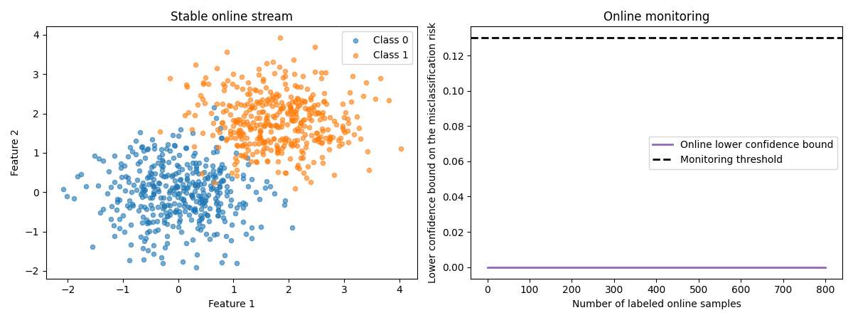
Monitor a stable stream
Now we monitor a stable online stream. Since the data distribution does not change, the online lower confidence bound should remain well below the monitoring threshold.
X_online_no_shift, y_online_no_shift = generate_gaussian_stream(
    n_samples=800,
    shift_type="stable",
    random_state=random_state + 2,
)

for start in range(0, len(X_online_no_shift), batch_size):
    stop = start + batch_size
    y_pred_batch = clf.predict(X_online_no_shift[start:stop])
    monitor_no_shift.update(y_online_no_shift[start:stop], y_pred_batch)

print(
    "No-shift scenario - harmful shift detected? "
    f"{monitor_no_shift.harmful_shift_detected}"
)

plot_monitoring_results(
    X_online_no_shift,
    y_online_no_shift,
    monitor_no_shift,
    threshold,
    title="Stable online stream",
)
Out:
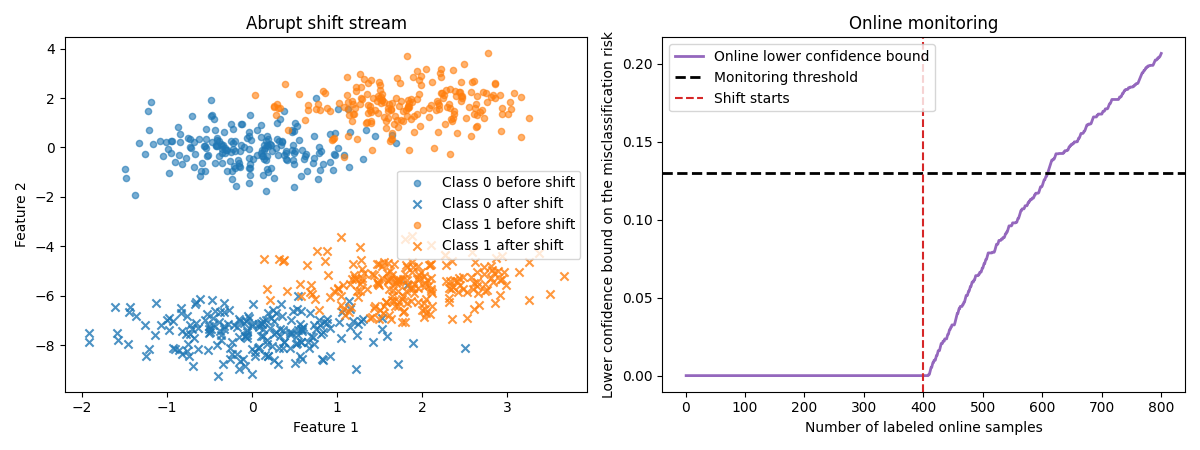
Monitor an abrupt shift
Now let us see what happens when an abrupt shift occurs in the middle of
the stream. The data distribution changes suddenly, and the lower
confidence bound eventually crosses the threshold. Note that there is no
need to call compute_threshold again: we can reuse the threshold
computed earlier (this also shows that any custom threshold can be passed
directly at instantiation).
X_online_abrupt, y_online_abrupt = generate_gaussian_stream(
    n_samples=800,
    shift_type="abrupt",
    prop_shift=prop_shift,
    random_state=random_state + 3,
)
shift_start_abrupt = int(len(y_online_abrupt) * (1 - prop_shift))

monitor_abrupt = RiskMonitoring(risk="accuracy", threshold=threshold)
for start in range(0, len(X_online_abrupt), batch_size):
    stop = start + batch_size
    y_pred_batch = clf.predict(X_online_abrupt[start:stop])
    monitor_abrupt.update(y_online_abrupt[start:stop], y_pred_batch)

print(
    "Abrupt-shift scenario - harmful shift detected? "
    f"{monitor_abrupt.harmful_shift_detected}"
)

plot_monitoring_results(
    X_online_abrupt,
    y_online_abrupt,
    monitor_abrupt,
    threshold,
    title="Abrupt shift stream",
    shift_start=shift_start_abrupt,
)
Out:
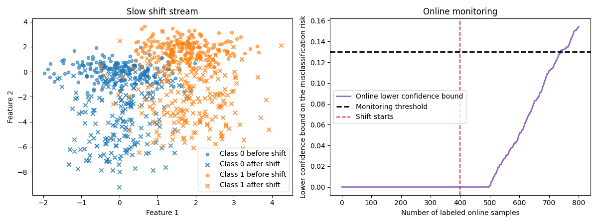
Monitor a slow drift
Finally, we create a slow drift. In that case the distribution evolves progressively, so the harmful shift is typically detected later than with an abrupt change.
X_online_slow, y_online_slow = generate_gaussian_stream(
    n_samples=800,
    shift_type="slow",
    prop_shift=prop_shift,
    random_state=random_state + 4,
)
shift_start_slow = int(len(y_online_slow) * (1 - prop_shift))

monitor_slow = RiskMonitoring(risk="accuracy", threshold=threshold)
for start in range(0, len(X_online_slow), batch_size):
    stop = start + batch_size
    y_pred_batch = clf.predict(X_online_slow[start:stop])
    monitor_slow.update(y_online_slow[start:stop], y_pred_batch)

print(
    "Slow-shift scenario - harmful shift detected? "
    f"{monitor_slow.harmful_shift_detected}"
)

plot_monitoring_results(
    X_online_slow,
    y_online_slow,
    monitor_slow,
    threshold,
    title="Slow shift stream",
    shift_start=shift_start_slow,
)
Out:
Interpret the scenarios
As expected, RiskMonitoring correctly does not fire any alarm on the
stable stream, detects the abrupt shift shortly after it occurs, and
eventually detects the slow drift once enough evidence has accumulated.
Total running time of the script: ( 0 minutes 5.505 seconds)
Download Python source code: plot_risk_monitoring.py