Note

Click here to download the full example code

Exchangeability testing on a fixed dataset

This quickstart demonstrates how to test exchangeability on a fixed dataset.

Guarantees provided by conformal prediction and risk control depend on the hypothesis that data is exchangeable. Verifying exchangeability before applying methods from MAPIE is therefore important. Typically, (split) conformal prediction, risk control, and calibration require data not seen during training, such as a split of the test data.

Note that for the exchangeability test to be valid, the order of samples in the fixed dataset must be representative of what will happen after deployment. Shuffling the data beforehand would trivially render the dataset exchangeable and hide any potential distribution shift.

Prepare the data

We first prepare the data and fit a classifier on the training data.

from sklearn.linear_model import LogisticRegression
from sklearn.model_selection import train_test_split

from mapie._example_utils import generate_gaussian_stream, plot_dataset
from mapie.classification import SplitConformalClassifier
from mapie.exchangeability_testing import FixedDatasetExchangeabilityTest

random_state = 42

X, y = generate_gaussian_stream(
    shift_type="stable",
    random_state=random_state,
)
X_train, X_test, y_train, y_test = train_test_split(
    X, y, test_size=0.3, random_state=random_state, shuffle=False
)

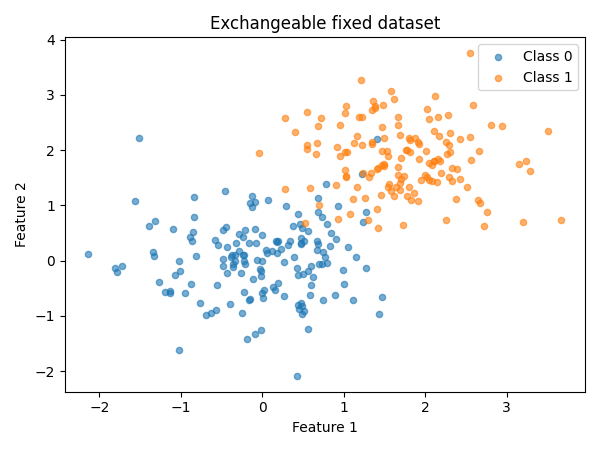
plot_dataset(
    X_test,
    y_test,
    title="Exchangeable fixed dataset",
)

classifier = LogisticRegression(random_state=random_state)
classifier.fit(X_train, y_train)

LogisticRegression(random_state=42)

In a Jupyter environment, please rerun this cell to show the HTML representation or trust the notebook.
On GitHub, the HTML representation is unable to render, please try loading this page with nbviewer.org.

Run the exchangeability test

Now we can test the exchangeability of the test dataset. By default, we use all available test methods. Method-specific parameters can be passed as a dictionary.

exchangeability_test = FixedDatasetExchangeabilityTest()
exchangeability_test.run(X_test, y_test)

print("Is the test dataset exchangeable?")
for test_name, is_exchangeable in exchangeability_test.is_exchangeable.items():
    print(f"{test_name}: {is_exchangeable}")

Out:

Is the test dataset exchangeable?
pvalue_permutation: True
permutation_binomial: True
permutation_binomial_mixture: True
permutation_aggressive: True
plugin_martingale: True
jumper_martingale: True

Continue with MAPIE

The test dataset is exchangeable. We can continue with MAPIE. Conformalization with a split of the test dataset will provide coverage guarantees on the remaining test data.

X_conformalize, X_test_new, y_conformalize, y_test_new = train_test_split(
    X_test, y_test, test_size=0.5, random_state=random_state
)

confidence_level = 0.95
mapie_classifier = SplitConformalClassifier(
    estimator=classifier, confidence_level=confidence_level, prefit=True
)
mapie_classifier.conformalize(X_conformalize, y_conformalize)
y_pred, y_pred_set = mapie_classifier.predict_set(X_test_new)

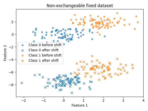
Create a non-exchangeable dataset

Now let us see what happens for a non-exchangeable fixed dataset. Here, an abrupt shift happens in the second part of the dataset.

X_test_abrupt, y_test_abrupt = generate_gaussian_stream(
    n_samples=len(X_test),
    shift_type="abrupt",
    prop_shift=0.5,
    random_state=random_state + 1,
)
shift_start_abrupt = int(len(y_test_abrupt) * 0.5)
plot_dataset(
    X_test_abrupt,
    y_test_abrupt,
    title="Non-exchangeable fixed dataset",
    shift_start=shift_start_abrupt,
)

exchangeability_test = FixedDatasetExchangeabilityTest()
exchangeability_test.run(X_test_abrupt, y_test_abrupt)

print("Is the shifted dataset exchangeable?")
for test_name, is_exchangeable in exchangeability_test.is_exchangeable.items():
    print(f"{test_name}: {is_exchangeable}")

Out:

Is the shifted dataset exchangeable?
pvalue_permutation: False
permutation_binomial: False
permutation_binomial_mixture: False
permutation_aggressive: False
plugin_martingale: False
jumper_martingale: True

Interpret the result

The shifted test dataset is not exchangeable: MAPIE cannot provide statistical guarantees on it, and more generally the classifier itself should not be trusted without further investigation.

Note that the jumper martingale fails to detect the non-exchangeability in this case. Itmostly reacts to one-sided p-value distortions (many consistently small p-values, or many consistently large ones). The shift creates both many very low and many very high p-values, the effects cancel out for the jumper martingale. More generally, this illustrates that no single test is perfect, and that it is important to use multiple tests to get a complete picture.

Total running time of the script: ( 0 minutes 8.169 seconds)

Download Python source code: plot_exchangeability_fixed_dataset.py

Download Jupyter notebook: plot_exchangeability_fixed_dataset.ipynb

Gallery generated by mkdocs-gallery