Logistic regression with Elastic net and minimax concave penalties

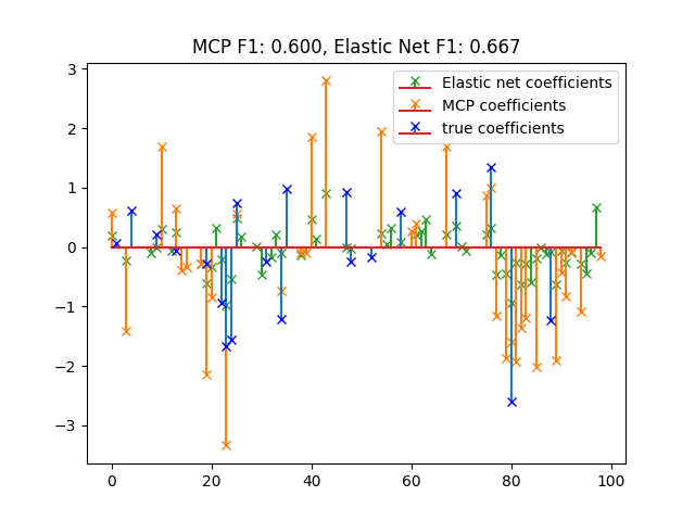
Illustrate the modularity of skglm by using GeneralizedLinearEstimator with one datafit and one penalty.

# Author: Pierre-Antoine Bannier

import numpy as np
from numpy.linalg import norm
import matplotlib.pyplot as plt

from sklearn.metrics import f1_score

from skglm import GeneralizedLinearEstimator
from skglm.datafits import Logistic
from skglm.penalties import L1_plus_L2, MCPenalty
from skglm.utils.data import make_correlated_data


n_samples, n_features = 50, 100
X, y, w_star = make_correlated_data(
    n_samples=n_samples, n_features=n_features, random_state=0)
y_ind = np.sign(y)

# standardize for MCP
X /= norm(X, axis=0) / np.sqrt(len(X))

# Split data in train set and test set
X_train, y_train = X[: n_samples // 2], y_ind[: n_samples // 2]
X_test, y_test = X[n_samples // 2:], y_ind[n_samples // 2:]


alpha = 0.005
gamma = 3.0
l1_ratio = 0.3
clf_enet = GeneralizedLinearEstimator(
    Logistic(),
    L1_plus_L2(alpha, l1_ratio),
)
y_pred_enet = clf_enet.fit(X_train, y_train).predict(X_test)
f1_score_enet = f1_score(y_test, y_pred_enet)

clf_mcp = GeneralizedLinearEstimator(
    Logistic(),
    MCPenalty(alpha, gamma),
)
y_pred_mcp = clf_mcp.fit(X_train, y_train).predict(X_test)
f1_score_mcp = f1_score(y_test, y_pred_mcp)


m, s, _ = plt.stem(
    np.where(clf_enet.coef_.ravel())[0],
    clf_enet.coef_[clf_enet.coef_ != 0],
    markerfmt="x",
    label="Elastic net coefficients",
)
plt.setp([m, s], color="#2ca02c")
m, s, _ = plt.stem(
    np.where(clf_mcp.coef_.ravel())[0],
    clf_mcp.coef_[clf_mcp.coef_ != 0],
    markerfmt="x",
    label="MCP coefficients",
)
plt.setp([m, s], color="#ff7f0e")
plt.stem(
    np.where(w_star)[0],
    w_star[w_star != 0],
    label="true coefficients",
    markerfmt="bx",
)

plt.legend(loc="best")
plt.title("MCP F1: %.3f, Elastic Net F1: %.3f" % (f1_score_mcp, f1_score_enet))
plt.show()