Use a pre-trained model¶

SplitConformalRegressor and ConformalizedQuantileRegressor are used to conformalize uncertainties for large models for which the cost of cross-validation is too high. Typically, neural networks rely on a single validation set.

In this example, we first fit a neural network on the training set. We then compute residuals on a validation set with the prefit=True parameter. Finally, we evaluate the model with prediction intervals on a testing set. In a second part, we will also show how to use the prefit method in the conformalized quantile regressor.

import warnings

import numpy as np
import scipy
from lightgbm import LGBMRegressor
from matplotlib import pyplot as plt
from numpy.typing import NDArray
from sklearn.neural_network import MLPRegressor

from mapie.metrics.regression import regression_coverage_score
from mapie.regression import ConformalizedQuantileRegressor, SplitConformalRegressor
from mapie.utils import train_conformalize_test_split

warnings.filterwarnings("ignore")

RANDOM_STATE = 1
confidence_level = 0.9

We start by defining a function that we will use to generate data. We then add random noise to the y values. Then we split the dataset to have a training, conformalize and test set.

def f(x: NDArray) -> NDArray:
    """Polynomial function used to generate one-dimensional data."""
    return np.array(5 * x + 5 * x**4 - 9 * x**2)


# Generate data
rng = np.random.default_rng(59)
sigma = 0.1
n_samples = 10000
X = np.linspace(0, 1, n_samples)
y = f(X) + rng.normal(0, sigma, n_samples)

# Train/conformalize/test split
(X_train, X_conformalize, X_test, y_train, y_conformalize, y_test) = (
    train_conformalize_test_split(
        X,
        y,
        train_size=0.8,
        conformalize_size=0.1,
        test_size=0.1,
        random_state=RANDOM_STATE,
    )
)

1. Use a neural network¶

1.1 Pre-train a neural network¶

For this example, we will train a MLPRegressor for SplitConformalRegressor.

# Train a MLPRegressor for SplitConformalRegressor
est_mlp = MLPRegressor(activation="relu", random_state=RANDOM_STATE)
est_mlp.fit(X_train.reshape(-1, 1), y_train)

MLPRegressor(random_state=1)

In a Jupyter environment, please rerun this cell to show the HTML representation or trust the notebook.
On GitHub, the HTML representation is unable to render, please try loading this page with nbviewer.org.

MLPRegressor

?Documentation for MLPRegressoriFitted

Parameters

	random_state random_state: int, RandomState instance, default=None Determines random number generation for weights and bias initialization, train-test split if early stopping is used, and batch sampling when solver='sgd' or 'adam'. Pass an int for reproducible results across multiple function calls. See :term:`Glossary <random_state>`.	1
	loss loss: {'squared_error', 'poisson'}, default='squared_error' The loss function to use when training the weights. Note that the "squared error" and "poisson" losses actually implement "half squares error" and "half poisson deviance" to simplify the computation of the gradient. Furthermore, the "poisson" loss internally uses a log-link (exponential as the output activation function) and requires ``y >= 0``. .. versionchanged:: 1.7 Added parameter `loss` and option 'poisson'.	'squared_error'
	hidden_layer_sizes hidden_layer_sizes: array-like of shape(n_layers - 2,), default=(100,) The ith element represents the number of neurons in the ith hidden layer.	(100,)
	activation activation: {'identity', 'logistic', 'tanh', 'relu'}, default='relu' Activation function for the hidden layer. - 'identity', no-op activation, useful to implement linear bottleneck, returns f(x) = x - 'logistic', the logistic sigmoid function, returns f(x) = 1 / (1 + exp(-x)). - 'tanh', the hyperbolic tan function, returns f(x) = tanh(x). - 'relu', the rectified linear unit function, returns f(x) = max(0, x)	'relu'
	solver solver: {'lbfgs', 'sgd', 'adam'}, default='adam' The solver for weight optimization. - 'lbfgs' is an optimizer in the family of quasi-Newton methods. - 'sgd' refers to stochastic gradient descent. - 'adam' refers to a stochastic gradient-based optimizer proposed by Kingma, Diederik, and Jimmy Ba For a comparison between Adam optimizer and SGD, see :ref:`sphx_glr_auto_examples_neural_networks_plot_mlp_training_curves.py`. Note: The default solver 'adam' works pretty well on relatively large datasets (with thousands of training samples or more) in terms of both training time and validation score. For small datasets, however, 'lbfgs' can converge faster and perform better.	'adam'
	alpha alpha: float, default=0.0001 Strength of the L2 regularization term. The L2 regularization term is divided by the sample size when added to the loss.	0.0001
	batch_size batch_size: int, default='auto' Size of minibatches for stochastic optimizers. If the solver is 'lbfgs', the regressor will not use minibatch. When set to "auto", `batch_size=min(200, n_samples)`.	'auto'
	learning_rate learning_rate: {'constant', 'invscaling', 'adaptive'}, default='constant' Learning rate schedule for weight updates. - 'constant' is a constant learning rate given by 'learning_rate_init'. - 'invscaling' gradually decreases the learning rate ``learning_rate_`` at each time step 't' using an inverse scaling exponent of 'power_t'. effective_learning_rate = learning_rate_init / pow(t, power_t) - 'adaptive' keeps the learning rate constant to 'learning_rate_init' as long as training loss keeps decreasing. Each time two consecutive epochs fail to decrease training loss by at least tol, or fail to increase validation score by at least tol if 'early_stopping' is on, the current learning rate is divided by 5. Only used when solver='sgd'.	'constant'
	learning_rate_init learning_rate_init: float, default=0.001 The initial learning rate used. It controls the step-size in updating the weights. Only used when solver='sgd' or 'adam'.	0.001
	power_t power_t: float, default=0.5 The exponent for inverse scaling learning rate. It is used in updating effective learning rate when the learning_rate is set to 'invscaling'. Only used when solver='sgd'.	0.5
	max_iter max_iter: int, default=200 Maximum number of iterations. The solver iterates until convergence (determined by 'tol') or this number of iterations. For stochastic solvers ('sgd', 'adam'), note that this determines the number of epochs (how many times each data point will be used), not the number of gradient steps.	200
	shuffle shuffle: bool, default=True Whether to shuffle samples in each iteration. Only used when solver='sgd' or 'adam'.	True
	tol tol: float, default=1e-4 Tolerance for the optimization. When the loss or score is not improving by at least ``tol`` for ``n_iter_no_change`` consecutive iterations, unless ``learning_rate`` is set to 'adaptive', convergence is considered to be reached and training stops.	0.0001
	verbose verbose: bool, default=False Whether to print progress messages to stdout.	False
	warm_start warm_start: bool, default=False When set to True, reuse the solution of the previous call to fit as initialization, otherwise, just erase the previous solution. See :term:`the Glossary <warm_start>`.	False
	momentum momentum: float, default=0.9 Momentum for gradient descent update. Should be between 0 and 1. Only used when solver='sgd'.	0.9
	nesterovs_momentum nesterovs_momentum: bool, default=True Whether to use Nesterov's momentum. Only used when solver='sgd' and momentum > 0.	True
	early_stopping early_stopping: bool, default=False Whether to use early stopping to terminate training when validation score is not improving. If set to True, it will automatically set aside ``validation_fraction`` of training data as validation and terminate training when validation score is not improving by at least ``tol`` for ``n_iter_no_change`` consecutive epochs. Only effective when solver='sgd' or 'adam'.	False
	validation_fraction validation_fraction: float, default=0.1 The proportion of training data to set aside as validation set for early stopping. Must be between 0 and 1. Only used if early_stopping is True.	0.1
	beta_1 beta_1: float, default=0.9 Exponential decay rate for estimates of first moment vector in adam, should be in [0, 1). Only used when solver='adam'.	0.9
	beta_2 beta_2: float, default=0.999 Exponential decay rate for estimates of second moment vector in adam, should be in [0, 1). Only used when solver='adam'.	0.999
	epsilon epsilon: float, default=1e-8 Value for numerical stability in adam. Only used when solver='adam'.	1e-08
	n_iter_no_change n_iter_no_change: int, default=10 Maximum number of epochs to not meet ``tol`` improvement. Only effective when solver='sgd' or 'adam'. .. versionadded:: 0.20	10
	max_fun max_fun: int, default=15000 Only used when solver='lbfgs'. Maximum number of function calls. The solver iterates until convergence (determined by ``tol``), number of iterations reaches max_iter, or this number of function calls. Note that number of function calls will be greater than or equal to the number of iterations for the MLPRegressor. .. versionadded:: 0.22	15000

Fitted attributes

Name	Type	Value
best_loss_ best_loss_: float The minimum loss reached by the solver throughout fitting. If `early_stopping=True`, this attribute is set to `None`. Refer to the `best_validation_score_` fitted attribute instead. Only accessible when solver='sgd' or 'adam'.	float64	0.005514
best_validation_score_ best_validation_score_: float or None The best validation score (i.e. R2 score) that triggered the early stopping. Only available if `early_stopping=True`, otherwise the attribute is set to `None`. Only accessible when solver='sgd' or 'adam'.	NoneType	None
coefs_ coefs_: list of shape (n_layers - 1,) The ith element in the list represents the weight matrix corresponding to layer i.	list	[array([[-1.24...0946927e-02]]), array([[ 2.21...1670389e-01]])]
intercepts_ intercepts_: list of shape (n_layers - 1,) The ith element in the list represents the bias vector corresponding to layer i + 1.	list	[array([-0.084... 0.23990212]), array([0.13100566])]
loss_ loss_: float The current loss computed with the loss function.	float64	0.005514
loss_curve_ loss_curve_: list of shape (`n_iter_`,) Loss value evaluated at the end of each training step. The ith element in the list represents the loss at the ith iteration. Only accessible when solver='sgd' or 'adam'.	list	[np.float64(0....9556609491883), np.float64(0....2715618366643), np.float64(0....8279988382778), np.float64(0....2511722280698), ...]
n_features_in_ n_features_in_: int Number of features seen during :term:`fit`. .. versionadded:: 0.24	int	1
n_iter_ n_iter_: int The number of iterations the solver has run.	int	44
n_layers_ n_layers_: int Number of layers.	int	3
n_outputs_ n_outputs_: int Number of outputs.	int	1
out_activation_ out_activation_: str Name of the output activation function.	str	'id...ty'
t_ t_: int The number of training samples seen by the solver during fitting. Mathematically equals `n_iters * X.shape[0]`, it means `time_step` and it is used by optimizer's learning rate scheduler.	int	352000
validation_scores_ validation_scores_: list of shape (`n_iter_`,) or None The score at each iteration on a held-out validation set. The score reported is the R2 score. Only available if `early_stopping=True`, otherwise the attribute is set to `None`. Only accessible when solver='sgd' or 'adam'.	NoneType	None

1.2 Use MAPIE to conformalize the models¶

We will now proceed to conformalize the models using MAPIE. To this aim, we set prefit=True so that we use the model that we already trained prior. We then predict using the test set and evaluate its coverage.

# Conformalize uncertainties on conformalize set
mapie = SplitConformalRegressor(
    estimator=est_mlp, confidence_level=confidence_level, prefit=True
)
mapie.conformalize(X_conformalize.reshape(-1, 1), y_conformalize)

# Evaluate prediction and coverage level on testing set
y_pred, y_pis = mapie.predict_interval(X_test.reshape(-1, 1))
coverage = regression_coverage_score(y_test, y_pis)[0]

1.3 Plot results¶

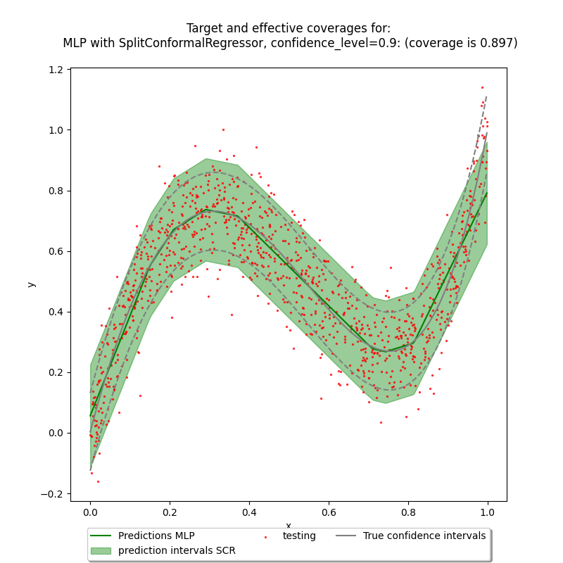
In order to view the results, we will plot the predictions of the the multi-layer perceptron (MLP) with their prediction intervals calculated with SplitConformalRegressor.

# Plot obtained prediction intervals on testing set
theoretical_semi_width = scipy.stats.norm.ppf(1 - confidence_level) * sigma
y_test_theoretical = f(X_test)
order = np.argsort(X_test)

plt.figure(figsize=(8, 8))
plt.plot(X_test[order], y_pred[order], label="Predictions MLP", color="green")
plt.fill_between(
    X_test[order],
    y_pis[:, 0, 0][order],
    y_pis[:, 1, 0][order],
    alpha=0.4,
    label="prediction intervals SCR",
    color="green",
)

plt.title(
    f"Target and effective coverages for:\n "
    f"MLP with SplitConformalRegressor, confidence_level={confidence_level}: "
    + f"(coverage is {coverage:.3f})\n"
)
plt.scatter(X_test, y_test, color="red", alpha=0.7, label="testing", s=2)
plt.plot(
    X_test[order],
    y_test_theoretical[order],
    color="gray",
    label="True confidence intervals",
)
plt.plot(
    X_test[order],
    y_test_theoretical[order] - theoretical_semi_width,
    color="gray",
    ls="--",
)
plt.plot(
    X_test[order],
    y_test_theoretical[order] + theoretical_semi_width,
    color="gray",
    ls="--",
)
plt.xlabel("x")
plt.ylabel("y")
plt.legend(
    loc="upper center", bbox_to_anchor=(0.5, -0.05), fancybox=True, shadow=True, ncol=3
)
plt.show()

Target and effective coverages for: MLP with SplitConformalRegressor, confidence_level=0.9: (coverage is 0.897)

2. Use LGBM models¶

2.1 Pre-train LGBM models¶

For this example, we will train multiple LGBMRegressor with a quantile objective as this is a requirement to perform conformalized quantile regression using ConformalizedQuantileRegressor. Note that the three estimators need to be trained at quantile values of (1+confidence_level)/2, (1-confidence_level)/2, 0.5).

# Train LGBMRegressor models for _MapieQuantileRegressor
list_estimators_cqr = []
for alpha_ in [(1 - confidence_level) / 2, (1 + confidence_level) / 2, 0.5]:
    estimator_ = LGBMRegressor(
        objective="quantile",
        alpha=alpha_,
    )
    estimator_.fit(X_train.reshape(-1, 1), y_train)
    list_estimators_cqr.append(estimator_)

Out:

[LightGBM] [Info] Auto-choosing col-wise multi-threading, the overhead of testing was 0.000062 seconds.
You can set `force_col_wise=true` to remove the overhead.
[LightGBM] [Info] Total Bins 255
[LightGBM] [Info] Number of data points in the train set: 8000, number of used features: 1
[LightGBM] [Info] Start training from score 0.148368
[LightGBM] [Info] Auto-choosing col-wise multi-threading, the overhead of testing was 0.000108 seconds.
You can set `force_col_wise=true` to remove the overhead.
[LightGBM] [Info] Total Bins 255
[LightGBM] [Info] Number of data points in the train set: 8000, number of used features: 1
[LightGBM] [Info] Start training from score 0.836819
[LightGBM] [Info] Auto-choosing col-wise multi-threading, the overhead of testing was 0.000051 seconds.
You can set `force_col_wise=true` to remove the overhead.
[LightGBM] [Info] Total Bins 255
[LightGBM] [Info] Number of data points in the train set: 8000, number of used features: 1
[LightGBM] [Info] Start training from score 0.505079

2.2 Use MAPIE to conformalize the models¶

We will now proceed to conformalize the models using MAPIE. To this aim, we set prefit=True so that we use the models that we already trained prior. We then predict using the test set and evaluate its coverage.

# Conformalize uncertainties on conformalize set
mapie_cqr = ConformalizedQuantileRegressor(
    list_estimators_cqr, confidence_level=0.9, prefit=True
)
mapie_cqr.conformalize(X_conformalize.reshape(-1, 1), y_conformalize)

# Evaluate prediction and coverage level on testing set
y_pred_cqr, y_pis_cqr = mapie_cqr.predict_interval(X_test.reshape(-1, 1))
coverage_cqr = regression_coverage_score(y_test, y_pis_cqr)[0]

2.3 Plot results¶

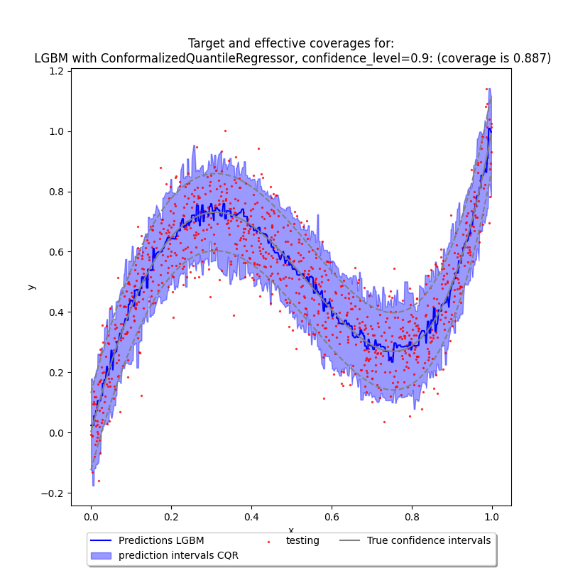
As fdor the MLP predictions, we plot the predictions of the LGBMRegressor with their prediction intervals calculated with ConformalizedQuantileRegressor.

# Plot obtained prediction intervals on testing set
theoretical_semi_width = scipy.stats.norm.ppf(1 - confidence_level) * sigma
y_test_theoretical = f(X_test)
order = np.argsort(X_test)

plt.figure(figsize=(8, 8))

plt.plot(X_test[order], y_pred_cqr[order], label="Predictions LGBM", color="blue")
plt.fill_between(
    X_test[order],
    y_pis_cqr[:, 0, 0][order],
    y_pis_cqr[:, 1, 0][order],
    alpha=0.4,
    label="prediction intervals CQR",
    color="blue",
)
plt.title(
    f"Target and effective coverages for:\n "
    f"LGBM with ConformalizedQuantileRegressor, confidence_level={confidence_level}: "
    + f"(coverage is {coverage_cqr:.3f})"
)
plt.scatter(X_test, y_test, color="red", alpha=0.7, label="testing", s=2)
plt.plot(
    X_test[order],
    y_test_theoretical[order],
    color="gray",
    label="True confidence intervals",
)
plt.plot(
    X_test[order],
    y_test_theoretical[order] - theoretical_semi_width,
    color="gray",
    ls="--",
)
plt.plot(
    X_test[order],
    y_test_theoretical[order] + theoretical_semi_width,
    color="gray",
    ls="--",
)
plt.xlabel("x")
plt.ylabel("y")
plt.legend(
    loc="upper center", bbox_to_anchor=(0.5, -0.05), fancybox=True, shadow=True, ncol=3
)
plt.show()

Target and effective coverages for: LGBM with ConformalizedQuantileRegressor, confidence_level=0.9: (coverage is 0.887)

Total running time of the script: ( 0 minutes 1.005 seconds)

Download Python source code: plot_prefit.py

Download Jupyter notebook: plot_prefit.ipynb

Gallery generated by mkdocs-gallery