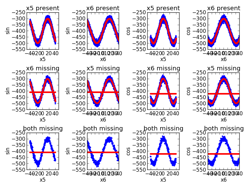
Plotting a multicolumn regression problem that includes missingness
An example plotting a simultaneous fit of the sine and cosine functions. There are two redundant predictors, each of which has independent and random missingness.
Out:
  Beginning forward pass
---------------------------------------------------------------------
iter  parent  var  knot  mse          terms  gcv       rsq    grsq
---------------------------------------------------------------------
0     -       -    -     4893.487156  1      4894.466  0.000  0.000
1     0       6    2137  2847.258070  5      2853.532  0.418  0.417
2     3       6    1882  1604.248646  7      1609.395  0.672  0.671
3     4       6    3981  1091.498983  9      1096.098  0.777  0.776
4     0       5    3872  865.753079  13     871.146  0.823  0.822
5     1       5    6251  677.545451  17     683.136  0.862  0.860
6     11      5    7295  529.897093  19     534.806  0.892  0.891
7     3       5    1687  429.659153  23     434.512  0.912  0.911
8     12      5    8217  356.980379  25     361.376  0.927  0.926
9     12      6    6100  311.466783  29     315.937  0.936  0.935
10    23      5    7367  305.774544  31     310.476  0.938  0.937
11    5       6    3688  302.715204  33     307.679  0.938  0.937
-------------------------------------------------------------------
Stopping Condition 2: Improvement below threshold
Beginning pruning pass
------------------------------------------------
iter  bf  terms  mse     gcv      rsq    grsq
------------------------------------------------
0     -   33     302.73  307.691  0.938  0.937
1     2   32     302.73  307.536  0.938  0.937
2     12  31     302.73  307.381  0.938  0.937
3     13  30     302.73  307.226  0.938  0.937
4     3   29     302.71  307.058  0.938  0.937
5     10  28     302.73  306.917  0.938  0.937
6     16  27     302.83  306.872  0.938  0.937
7     30  26     303.00  306.881  0.938  0.937
8     32  25     303.26  306.990  0.938  0.937
9     15  24     303.80  307.382  0.938  0.937
10    25  23     305.32  308.772  0.938  0.937
11    1   22     306.62  309.932  0.937  0.937
12    31  21     309.57  312.748  0.937  0.936
13    29  20     314.07  317.136  0.936  0.935
14    19  19     322.35  325.336  0.934  0.934
15    22  18     337.54  340.500  0.931  0.930
16    6   17     347.58  350.448  0.929  0.928
17    28  16     361.15  363.944  0.926  0.926
18    24  15     371.25  373.935  0.924  0.924
19    27  14     439.31  442.265  0.910  0.910
20    7   13     465.62  468.521  0.905  0.904
21    21  12     570.82  574.085  0.883  0.883
22    5   11     613.94  617.143  0.875  0.874
23    18  10     766.50  770.116  0.843  0.843
24    8   9      941.18  945.144  0.808  0.807
25    14  8      1153.75  1158.031  0.764  0.763
26    9   7      1376.30  1380.712  0.719  0.718
27    17  6      1780.93  1785.752  0.636  0.635
28    20  5      2192.81  2197.638  0.552  0.551
29    26  4      2561.68  2566.044  0.477  0.476
30    11  3      3302.02  3305.984  0.325  0.325
31    4   2      3745.34  3747.962  0.235  0.234
32    23  1      4893.49  4894.466  0.000  0.000
--------------------------------------------------
Selected iteration: 0
Forward Pass
---------------------------------------------------------------------
iter  parent  var  knot  mse          terms  gcv       rsq    grsq
---------------------------------------------------------------------
0     -       -    -     4893.487156  1      4894.466  0.000  0.000
1     0       6    2137  2847.258070  5      2853.532  0.418  0.417
2     3       6    1882  1604.248646  7      1609.395  0.672  0.671
3     4       6    3981  1091.498983  9      1096.098  0.777  0.776
4     0       5    3872  865.753079   13     871.146   0.823  0.822
5     1       5    6251  677.545451   17     683.136   0.862  0.860
6     11      5    7295  529.897093   19     534.806   0.892  0.891
7     3       5    1687  429.659153   23     434.512   0.912  0.911
8     12      5    8217  356.980379   25     361.376   0.927  0.926
9     12      6    6100  311.466783   29     315.937   0.936  0.935
10    23      5    7367  305.774544   31     310.476   0.938  0.937
11    5       6    3688  302.715204   33     307.679   0.938  0.937
---------------------------------------------------------------------
Stopping Condition 2: Improvement below threshold

Pruning Pass
--------------------------------------------------
iter  bf  terms  mse      gcv       rsq    grsq
--------------------------------------------------
0     -   33     302.73   307.691   0.938  0.937
1     2   32     302.73   307.536   0.938  0.937
2     12  31     302.73   307.381   0.938  0.937
3     13  30     302.73   307.226   0.938  0.937
4     3   29     302.71   307.058   0.938  0.937
5     10  28     302.73   306.917   0.938  0.937
6     16  27     302.83   306.872   0.938  0.937
7     30  26     303.00   306.881   0.938  0.937
8     32  25     303.26   306.990   0.938  0.937
9     15  24     303.80   307.382   0.938  0.937
10    25  23     305.32   308.772   0.938  0.937
11    1   22     306.62   309.932   0.937  0.937
12    31  21     309.57   312.748   0.937  0.936
13    29  20     314.07   317.136   0.936  0.935
14    19  19     322.35   325.336   0.934  0.934
15    22  18     337.54   340.500   0.931  0.930
16    6   17     347.58   350.448   0.929  0.928
17    28  16     361.15   363.944   0.926  0.926
18    24  15     371.25   373.935   0.924  0.924
19    27  14     439.31   442.265   0.910  0.910
20    7   13     465.62   468.521   0.905  0.904
21    21  12     570.82   574.085   0.883  0.883
22    5   11     613.94   617.143   0.875  0.874
23    18  10     766.50   770.116   0.843  0.843
24    8   9      941.18   945.144   0.808  0.807
25    14  8      1153.75  1158.031  0.764  0.763
26    9   7      1376.30  1380.712  0.719  0.718
27    17  6      1780.93  1785.752  0.636  0.635
28    20  5      2192.81  2197.638  0.552  0.551
29    26  4      2561.68  2566.044  0.477  0.476
30    11  3      3302.02  3305.984  0.325  0.325
31    4   2      3745.34  3747.962  0.235  0.234
32    23  1      4893.49  4894.466  0.000  0.000
--------------------------------------------------
Selected iteration: 0

Earth Model
---------------------------------------------------------------------------------------------------------------------------------------------------------------
Basis Function                                                                                                           Pruned  Coefficient 0  Coefficient 1
---------------------------------------------------------------------------------------------------------------------------------------------------------------
(Intercept)                                                                                                              No      -5.32206e+09   1.19712e+10
present(x6)                                                                                                              No      1.93529e+09    -4.35316e+09
missing(x6)                                                                                                              No      2.90294e+09    -6.52973e+09
C(x6|s=+1,-13.0806,-0.196727,11.4609)*present(x6)                                                                        No      3.39758        -5.46026
C(x6|s=-1,-13.0806,-0.196727,11.4609)*present(x6)                                                                        No      -1.66364       -10.5413
C(x6|s=+1,11.4609,23.1185,23.8585)*C(x6|s=+1,-13.0806,-0.196727,11.4609)*present(x6)                                     No      -0.425959      0.166173
C(x6|s=-1,11.4609,23.1185,23.8585)*C(x6|s=+1,-13.0806,-0.196727,11.4609)*present(x6)                                     No      0.388521       -0.0691114
C(x6|s=+1,-32.9814,-25.9644,-13.0806)*C(x6|s=-1,-13.0806,-0.196727,11.4609)*present(x6)                                  No      -0.481603      -0.0625639
C(x6|s=-1,-32.9814,-25.9644,-13.0806)*C(x6|s=-1,-13.0806,-0.196727,11.4609)*present(x6)                                  No      0.26819        0.319225
present(x5)                                                                                                              No      2.41912e+09    -5.44144e+09
missing(x5)                                                                                                              No      2.41912e+09    -5.44144e+09
C(x5|s=+1,-9.38452,1.36818,14.8996)*present(x5)                                                                          No      0.121137       -10.2913
C(x5|s=-1,-9.38452,1.36818,14.8996)*present(x5)                                                                          No      -2.91523       -0.483027
present(x5)*present(x6)                                                                                                  No      9.67647e+08    -2.17658e+09
missing(x5)*present(x6)                                                                                                  No      9.67647e+08    -2.17658e+09
C(x5|s=+1,-19.348,1.389,13.869)*present(x5)*present(x6)                                                                  No      -5.21392       6.62229
C(x5|s=-1,-19.348,1.389,13.869)*present(x5)*present(x6)                                                                  No      9.22985        -6.41773
C(x5|s=+1,14.8996,28.4311,34.2832)*C(x5|s=+1,-9.38452,1.36818,14.8996)*present(x5)                                       No      -0.229284      0.365081
C(x5|s=-1,14.8996,28.4311,34.2832)*C(x5|s=+1,-9.38452,1.36818,14.8996)*present(x5)                                       No      0.444821       -0.129529
present(x5)*C(x6|s=+1,-13.0806,-0.196727,11.4609)*present(x6)                                                            No      3.81312        -0.595014
missing(x5)*C(x6|s=+1,-13.0806,-0.196727,11.4609)*present(x6)                                                            No      -0.416023      -4.86417
C(x5|s=+1,13.869,26.349,33.2422)*present(x5)*C(x6|s=+1,-13.0806,-0.196727,11.4609)*present(x6)                           No      0.247209       -0.335965
C(x5|s=-1,13.869,26.349,33.2422)*present(x5)*C(x6|s=+1,-13.0806,-0.196727,11.4609)*present(x6)                           No      -0.42469       0.0927334
C(x5|s=+1,-35.584,-31.0829,-25.61)*C(x5|s=-1,-9.38452,1.36818,14.8996)*present(x5)                                       No      -0.417321      -0.122234
C(x5|s=-1,-35.584,-31.0829,-25.61)*C(x5|s=-1,-9.38452,1.36818,14.8996)*present(x5)                                       No      0.199904       0.309103
present(x6)*C(x5|s=-1,-9.38452,1.36818,14.8996)*present(x5)                                                              No      -5.554         7.50276
missing(x6)*C(x5|s=-1,-9.38452,1.36818,14.8996)*present(x5)                                                              No      2.63895        -7.98618
C(x6|s=+1,-35.0155,-30.0326,4.9814)*present(x6)*C(x5|s=-1,-9.38452,1.36818,14.8996)*present(x5)                          No      0.434228       0.0633731
C(x6|s=-1,-35.0155,-30.0326,4.9814)*present(x6)*C(x5|s=-1,-9.38452,1.36818,14.8996)*present(x5)                          No      -0.266897      -0.316667
C(x5|s=+1,-25.61,-20.1372,-9.38452)*C(x5|s=+1,-35.584,-31.0829,-25.61)*C(x5|s=-1,-9.38452,1.36818,14.8996)*present(x5)   No      0.0011487      0.00313568
C(x5|s=-1,-25.61,-20.1372,-9.38452)*C(x5|s=+1,-35.584,-31.0829,-25.61)*C(x5|s=-1,-9.38452,1.36818,14.8996)*present(x5)   No      -0.00453544    -0.00781131
C(x6|s=+1,23.8585,24.5984,32.2969)*C(x6|s=+1,11.4609,23.1185,23.8585)*C(x6|s=+1,-13.0806,-0.196727,11.4609)*present(x6)  No      0.00825191     0.00633597
C(x6|s=-1,23.8585,24.5984,32.2969)*C(x6|s=+1,11.4609,23.1185,23.8585)*C(x6|s=+1,-13.0806,-0.196727,11.4609)*present(x6)  No      -0.0136051     -0.00110534
---------------------------------------------------------------------------------------------------------------------------------------------------------------
MSE: 296.2991, GCV: 301.1581, RSQ: 0.9395, GRSQ: 0.9385
import numpy
import matplotlib.pyplot as plt

from pyearth import Earth

# Create some fake data
numpy.random.seed(2)
m = 10000
n = 10
X = 80 * numpy.random.uniform(size=(m, n)) - 40
X[:, 5] = X[:, 6] + numpy.random.normal(0, .1, m)
y1 = 100 * \
    (numpy.sin((X[:, 5] + X[:, 6]) / 20) - 4.0) + \
    10 * numpy.random.normal(size=m)
y2 = 100 * \
    (numpy.cos((X[:, 5] + X[:, 6]) / 20) - 4.0) + \
    10 * numpy.random.normal(size=m)
y = numpy.concatenate([y1[:, None], y2[:, None]], axis=1)
missing = numpy.random.binomial(1, .2, (m, n)).astype(bool)
X_full = X.copy()
X[missing] = None
idx5 = (1 - missing[:, 5]).astype(bool)
idx6 = (1 - missing[:, 6]).astype(bool)

# Fit an Earth model
model = Earth(max_degree=5, minspan_alpha=.5, allow_missing=True,
              enable_pruning=True, thresh=.001, smooth=True,
              verbose=True)
model.fit(X, y)

# Print the model
print(model.trace())
print(model.summary())

# Plot the model
y_hat = model.predict(X)
fig = plt.figure()

for j in [0, 1]:
    ax1 = fig.add_subplot(3, 4, 1 + 2*j)
    ax1.plot(X_full[idx5, 5], y[idx5, j], 'b.')
    ax1.plot(X_full[idx5, 5], y_hat[idx5, j], 'r.')
    ax1.set_xlim(-40, 40)
    ax1.set_title('x5 present')
    ax1.set_xlabel('x5')
    ax1.set_ylabel('sin' if j == 0 else 'cos')

    ax2 = fig.add_subplot(3, 4, 2 + 2*j)
    ax2.plot(X_full[idx6, 6], y[idx6, j], 'b.')
    ax2.plot(X_full[idx6, 6], y_hat[idx6, j], 'r.')
    ax2.set_xlim(-40, 40)
    ax2.set_title('x6 present')
    ax2.set_xlabel('x6')
    ax2.set_ylabel('sin' if j == 0 else 'cos')

    ax3 = fig.add_subplot(3, 4, 5 + 2*j, sharex=ax1)
    ax3.plot(X_full[~idx6, 5], y[~idx6, j], 'b.')
    ax3.plot(X_full[~idx6, 5], y_hat[~idx6, j], 'r.')
    ax3.set_title('x6 missing')
    ax3.set_xlabel('x5')
    ax3.set_ylabel('sin' if j == 0 else 'cos')

    ax4 = fig.add_subplot(3, 4, 6 + 2*j, sharex=ax2)
    ax4.plot(X_full[~idx5, 6], y[~idx5, j], 'b.')
    ax4.plot(X_full[~idx5, 6], y_hat[~idx5, j], 'r.')
    ax4.set_title('x5 missing')
    ax4.set_xlabel('x6')
    ax4.set_ylabel('sin' if j == 0 else 'cos')

    ax5 = fig.add_subplot(3, 4, 9 + 2*j, sharex=ax1)
    ax5.plot(X_full[(~idx6) & (~idx5), 5], y[(~idx6) & (~idx5), j], 'b.')
    ax5.plot(X_full[(~idx6) & (~idx5), 5], y_hat[(~idx6) & (~idx5), j], 'r.')
    ax5.set_title('both missing')
    ax5.set_xlabel('x5')
    ax5.set_ylabel('sin' if j == 0 else 'cos')

    ax6 = fig.add_subplot(3, 4, 10 + 2*j, sharex=ax2)
    ax6.plot(X_full[(~idx6) & (~idx5), 6], y[(~idx6) & (~idx5), j], 'b.')
    ax6.plot(X_full[(~idx6) & (~idx5), 6], y_hat[(~idx6) & (~idx5), j], 'r.')
    ax6.set_title('both missing')
    ax6.set_xlabel('x6')
    ax6.set_ylabel('sin' if j == 0 else 'cos')

fig.tight_layout()
plt.show()
Total running time of the script: (0 minutes 59.852 seconds)
Download Python source code:
plot_multicolumn.py
Download IPython notebook:
plot_multicolumn.ipynb