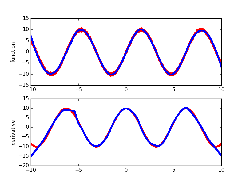
Plotting derivatives of simple sine function
A simple example plotting a fit of the sine function and the derivatives computed by Earth.
Out:
  Forward Pass
-----------------------------------------------------------------
iter  parent  var  knot  mse        terms  gcv     rsq    grsq
-----------------------------------------------------------------
0     -       -    -     47.918854  1      47.928  0.000  0.000
1     0       6    6267  44.373430  3      44.427  0.074  0.073
2     1       6    910   36.297242  5      36.377  0.243  0.241
3     2       6    5630  21.514715  7      21.584  0.551  0.550
4     0       6    2975  10.917076  9      10.963  0.772  0.771
5     8       6    2991  3.708183   11     3.728   0.923  0.922
6     7       6    2577  1.509533   13     1.519   0.968  0.968
7     1       6    1569  0.882026   15     0.888   0.982  0.981
8     2       6    264   0.577276   17     0.582   0.988  0.988
9     0       6    4442  0.313841   19     0.317   0.993  0.993
10    0       6    4497  0.232471   21     0.235   0.995  0.995
11    20      6    4242  0.190910   23     0.193   0.996  0.996
-----------------------------------------------------------------
Stopping Condition 2: Improvement below threshold

Pruning Pass
----------------------------------------------
iter  bf  terms  mse    gcv     rsq    grsq
----------------------------------------------
0     -   23     0.19   0.193   0.996  0.996
1     10  22     0.19   0.193   0.996  0.996
2     20  21     0.19   0.193   0.996  0.996
3     15  20     0.19   0.193   0.996  0.996
4     8   19     0.19   0.193   0.996  0.996
5     18  18     0.19   0.193   0.996  0.996
6     14  17     0.19   0.192   0.996  0.996
7     12  16     0.19   0.193   0.996  0.996
8     5   15     0.19   0.193   0.996  0.996
9     22  14     0.19   0.195   0.996  0.996
10    6   13     0.20   0.196   0.996  0.996
11    1   12     0.24   0.239   0.995  0.995
12    4   11     0.24   0.242   0.995  0.995
13    7   10     0.29   0.290   0.994  0.994
14    3   9      0.52   0.523   0.989  0.989
15    13  8      0.68   0.682   0.986  0.986
16    11  7      9.35   9.382   0.805  0.804
17    19  6      17.56  17.603  0.634  0.633
18    17  5      20.15  20.192  0.580  0.579
19    16  4      26.45  26.491  0.448  0.447
20    2   3      32.32  32.360  0.326  0.325
21    21  2      42.58  42.615  0.111  0.111
22    9   1      47.92  47.928  0.000  0.000
----------------------------------------------
Selected iteration: 6

Earth Model
--------------------------------------------------------------------------------------------------
Basis Function                                                               Pruned  Coefficient
--------------------------------------------------------------------------------------------------
(Intercept)                                                                  No      44.8098
C(x6|s=+1,-5.41239,-5.16768,-4.67412)                                        No      -26.6867
C(x6|s=-1,-5.41239,-5.16768,-4.67412)                                        No      31.9844
C(x6|s=+1,-0.137739,0.751892,1.25163)*C(x6|s=+1,-5.41239,-5.16768,-4.67412)  No      0.909836
C(x6|s=-1,-0.137739,0.751892,1.25163)*C(x6|s=+1,-5.41239,-5.16768,-4.67412)  No      -1.83328
C(x6|s=+1,-6.49945,-5.65709,-5.41239)*C(x6|s=-1,-5.41239,-5.16768,-4.67412)  No      -2.86683
C(x6|s=-1,-6.49945,-5.65709,-5.41239)*C(x6|s=-1,-5.41239,-5.16768,-4.67412)  No      3.05546
C(x6|s=+1,3.01553,4.27971,4.81202)                                           No      -5.61853
C(x6|s=-1,3.01553,4.27971,4.81202)                                           Yes     None
C(x6|s=+1,-1.70957,-1.02737,-0.137739)*C(x6|s=-1,3.01553,4.27971,4.81202)    No      1.74983
C(x6|s=-1,-1.70957,-1.02737,-0.137739)*C(x6|s=-1,3.01553,4.27971,4.81202)    Yes     None
C(x6|s=+1,6.35128,7.35822,8.67854)*C(x6|s=+1,3.01553,4.27971,4.81202)        No      -6.60667
C(x6|s=-1,6.35128,7.35822,8.67854)*C(x6|s=+1,3.01553,4.27971,4.81202)        No      4.12412
C(x6|s=+1,-3.28616,-2.39176,-1.70957)*C(x6|s=+1,-5.41239,-5.16768,-4.67412)  No      2.62654
C(x6|s=-1,-3.28616,-2.39176,-1.70957)*C(x6|s=+1,-5.41239,-5.16768,-4.67412)  Yes     None
C(x6|s=+1,-8.6707,-7.34181,-6.49945)*C(x6|s=-1,-5.41239,-5.16768,-4.67412)   Yes     None
C(x6|s=-1,-8.6707,-7.34181,-6.49945)*C(x6|s=-1,-5.41239,-5.16768,-4.67412)   No      3.58191
C(x6|s=+1,1.25163,1.75136,3.01553)                                           No      -9.68315
C(x6|s=-1,1.25163,1.75136,3.01553)                                           Yes     None
C(x6|s=+1,4.81202,5.34433,6.35128)                                           No      -12.1327
C(x6|s=-1,4.81202,5.34433,6.35128)                                           Yes     None
C(x6|s=+1,-4.67412,-4.18056,-3.28616)*C(x6|s=-1,4.81202,5.34433,6.35128)     No      2.68856
C(x6|s=-1,-4.67412,-4.18056,-3.28616)*C(x6|s=-1,4.81202,5.34433,6.35128)     No      -3.3853
--------------------------------------------------------------------------------------------------
MSE: 0.1448, GCV: 0.1460, RSQ: 0.9970, GRSQ: 0.9970
import numpy
import matplotlib.pyplot as plt

from pyearth import Earth

# Create some fake data
numpy.random.seed(2)
m = 10000
n = 10
X = 20 * numpy.random.uniform(size=(m, n)) - 10
y = 10*numpy.sin(X[:, 6]) + 0.25*numpy.random.normal(size=m)

# Compute the known true derivative with respect to the predictive variable
y_prime = 10*numpy.cos(X[:, 6])

# Fit an Earth model
model = Earth(max_degree=2, minspan_alpha=.5, smooth=True)
model.fit(X, y)

# Print the model
print(model.trace())
print(model.summary())

# Get the predicted values and derivatives
y_hat = model.predict(X)
y_prime_hat = model.predict_deriv(X, 'x6')

# Plot true and predicted function values and derivatives
# for the predictive variable
plt.subplot(211)
plt.plot(X[:, 6], y, 'r.')
plt.plot(X[:, 6], y_hat, 'b.')
plt.ylabel('function')
plt.subplot(212)
plt.plot(X[:, 6], y_prime, 'r.')
plt.plot(X[:, 6], y_prime_hat[:, 0], 'b.')
plt.ylabel('derivative')
plt.show()
Total running time of the script: (0 minutes 7.862 seconds)
Download Python source code:
plot_derivatives.py
Download IPython notebook:
plot_derivatives.ipynb