Comparison of lifelines with skglm for survival analysis

This example shows that skglm fits a Cox model exactly as lifelines but with x100 less time.

Data

Let’s first generate synthetic data on which to run the Cox estimator, using skglm data utils.

from skglm.utils.data import make_dummy_survival_data

n_samples, n_features = 500, 100
X, y = make_dummy_survival_data(
    n_samples, n_features,
    normalize=True,
    random_state=0
)

tm, s = y[:, 0], y[:, 1]

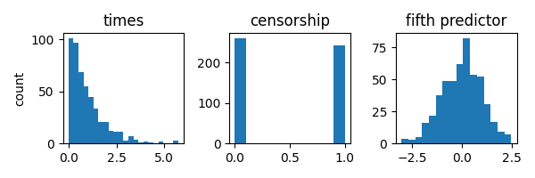
The synthetic data has the following properties:

• X is the matrix of predictors, generated using standard normal distribution with Toeplitz covariance.

• tm is the vector of occurrence times which follows a Weibull(1) distribution

• s indicates the observations censorship and follows a Bernoulli(0.5) distribution

Let’s inspect the data quickly:

import matplotlib.pyplot as plt

fig, axes = plt.subplots(
    1, 3,
    figsize=(6, 2),
    tight_layout=True,
)

dists = (tm, s, X[:, 5])
axes_title = ("times", "censorship", "fifth predictor")

for idx, (dist, name) in enumerate(zip(dists, axes_title)):
    axes[idx].hist(dist, bins="auto")
    axes[idx].set_title(name)

_ = axes[0].set_ylabel("count")

Fitting the Cox Estimator

After generating the synthetic data, we can now fit a L1-regularized Cox estimator. Todo so, we need to combine a Cox datafit and a `\ell_1` penalty and solve the resulting problem using skglm Proximal Newton solver ProxNewton. We set the intensity of the `\ell_1` regularization to alpha=1e-2.

from skglm.datafits import Cox
from skglm.penalties import L1
from skglm.solvers import ProxNewton

from skglm.utils.jit_compilation import compiled_clone

# regularization intensity
alpha = 1e-2

# skglm internals: init datafit and penalty
datafit = compiled_clone(Cox())
penalty = compiled_clone(L1(alpha))

datafit.initialize(X, y)

# init solver
solver = ProxNewton(fit_intercept=False, max_iter=50)

# solve the problem
w_sk = solver.solve(X, y, datafit, penalty)[0]

For this data a regularization value a relatively sparse solution is found:

print(
    "Number of nonzero coefficients in solution: "
    f"{(w_sk != 0).sum()} out of {len(w_sk)}."
)

Number of nonzero coefficients in solution: 66 out of 100.

Let’s solve the problem with lifelines through its CoxPHFitter estimator and compare the objectives found by the two packages.

import numpy as np
import pandas as pd
from lifelines import CoxPHFitter

# format data
stacked_y_X = np.hstack((y, X))
df = pd.DataFrame(stacked_y_X)

# fit lifelines estimator
lifelines_estimator = CoxPHFitter(penalizer=alpha, l1_ratio=1.).fit(
    df,
    duration_col=0,
    event_col=1
)
w_ll = lifelines_estimator.params_.values

Check that both solvers find solutions having the same objective value:

obj_sk = datafit.value(y, w_sk, X @ w_sk) + penalty.value(w_sk)
obj_ll = datafit.value(y, w_ll, X @ w_ll) + penalty.value(w_ll)

print(f"Objective skglm: {obj_sk:.6f}")
print(f"Objective lifelines: {obj_ll:.6f}")
print(f"Difference: {(obj_sk - obj_ll):.2e}")

Objective skglm: 2.494576
Objective lifelines: 2.494576
Difference: 1.47e-10

We can do the same to check how close the two solutions are.

print(f"Euclidean distance between solutions: {np.linalg.norm(w_sk - w_ll):.3e}")

Euclidean distance between solutions: 3.373e-04

Timing comparison

Now that we checked that both skglm and lifelines yield the same results, let’s compare their execution time. To get the evolution of the suboptimality (objective - optimal objective) we run both estimators with increasing number of iterations.

import time
import warnings

warnings.filterwarnings('ignore')

# where to save records
records = {
    "skglm": {"times": [], "objs": []},
    "lifelines": {"times": [], "objs": []},
}

# time skglm
max_runs = 20
for n_iter in range(1, max_runs + 1):
    solver.max_iter = n_iter

    start = time.perf_counter()
    w = solver.solve(X, y, datafit, penalty)[0]
    end = time.perf_counter()

    records["skglm"]["objs"].append(
        datafit.value(y, w, X @ w) + penalty.value(w)
    )
    records["skglm"]["times"].append(end - start)

# time lifelines
max_runs = 50
for n_iter in list(range(10)) + list(range(10, max_runs + 1, 5)):
    start = time.perf_counter()
    lifelines_estimator.fit(
        df,
        duration_col=0,
        event_col=1,
        fit_options={"max_steps": n_iter},
    )
    end = time.perf_counter()

    w = lifelines_estimator.params_.values

    records["lifelines"]["objs"].append(
        datafit.value(y, w, X @ w) + penalty.value(w)
    )
    records["lifelines"]["times"].append(end - start)


# cast records as numpy array
for idx, label in enumerate(("skglm", "lifelines")):
    for metric in ("objs", "times"):
        records[label][metric] = np.asarray(records[label][metric])

Results

fig, ax = plt.subplots(1, 1, tight_layout=True, figsize=(6, 3))
solvers = ("skglm", "lifelines")

optimal_obj = min(records[solver]["objs"].min() for solver in solvers)

# plot evolution of suboptimality
for solver in solvers:
    ax.semilogy(
        records[solver]["times"],
        records[solver]["objs"] - optimal_obj,
        label=solver,
        marker='o',
    )
ax.legend()
ax.set_title("Time to fit a Cox model")

ax.set_ylabel("objective suboptimality")
_ = ax.set_xlabel("time in seconds")

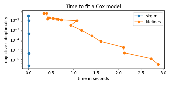
According to printed ratio, using skglm we get the same result as lifelines with more than x100 less time!

speed_up = records["lifelines"]["times"][-1] / records["skglm"]["times"][-1]
print(f"speed up ratio: {speed_up:.0f}")

speed up ratio: 797

Efron estimate

The previous results, namely closeness of solutions and timings, can be extended to the case of handling tied observation with the Efron estimate.

Let’s start by generating data with tied observations. This can be achieved by passing in a with_ties=True to make_dummy_survival_data function.

X, y = make_dummy_survival_data(
    n_samples, n_features,
    normalize=True,
    with_ties=True,
    random_state=0
)
tm, s = y[:, 0], y[:, 1]

# check the data has tied observations
print(f"Number of unique times {len(np.unique(tm))} out of {n_samples}")

Number of unique times 51 out of 500

It is straightforward to fit an `\ell_1` Cox estimator with the Efron estimate. We only need to pass in use_efron=True to the Cox datafit.

# ensure using Efron estimate
datafit = compiled_clone(Cox(use_efron=True))
datafit.initialize(X, y)

# solve the problem
solver = ProxNewton(fit_intercept=False, max_iter=50)
w_sk = solver.solve(X, y, datafit, penalty)[0]

Again a relatively sparse solution is found:

print(
    "Number of nonzero coefficients in solution: "
    f"{(w_sk != 0).sum()} out of {len(w_sk)}."
)

Number of nonzero coefficients in solution: 82 out of 100.

Let’s do the same with lifelines and compare the results

# format data
stacked_tm_s_X = np.hstack((tm[:, None], s[:, None], X))
df = pd.DataFrame(stacked_tm_s_X)

# fit lifelines estimator on the new data
lifelines_estimator = CoxPHFitter(penalizer=alpha, l1_ratio=1.).fit(
    df,
    duration_col=0,
    event_col=1
)
w_ll = lifelines_estimator.params_.values

# Check that both solvers find solutions with the same objective value
obj_sk = datafit.value(y, w_sk, X @ w_sk) + penalty.value(w_sk)
obj_ll = datafit.value(y, w_ll, X @ w_ll) + penalty.value(w_ll)

print(f"Objective skglm: {obj_sk:.6f}")
print(f"Objective lifelines: {obj_ll:.6f}")
print(f"Difference: {(obj_sk - obj_ll):.2e}")

# Check that both solutions are close
print(f"Euclidean distance between solutions: {np.linalg.norm(w_sk - w_ll):.3e}")

Objective skglm: 2.501289
Objective lifelines: 2.501289
Difference: -1.59e-09
Euclidean distance between solutions: 4.046e-04

Finally, let’s compare the timings of both solvers

# time skglm
start = time.perf_counter()
solver.solve(X, y, datafit, penalty)[0]
end = time.perf_counter()

total_time_skglm = end - start

# time lifelines
lifelines_estimator = CoxPHFitter(penalizer=alpha, l1_ratio=1.)

start = time.perf_counter()
lifelines_estimator.fit(
    df,
    duration_col=0,
    event_col=1
)
end = time.perf_counter()

total_time_lifelines = end - start

# deduce speed up ratio
speed_up = total_time_lifelines / total_time_skglm
print(f"speed up ratio: {speed_up:.0f}")

speed up ratio: 819

As shown by the last print, we still preserve the x100 ratio speed up even for the Efron estimate.