Confidence intervals versus observed prediction error
Each point below is a held-out observation. The horizontal coordinate is the
absolute residual, \(|y_i - \hat y_i|\); the vertical coordinate is the
approximate 95% confidence-interval half-width,
\(1.96\sqrt{\max(\widehat{V}_{IJ,i}, 0)}\). All models use 2,000 estimators
and calibrate=False. Negative raw IJ variances are clipped only to compute
the square root; each caption reports their number. A zero width caused by
clipping is not evidence of certainty.
The dashed diagonal marks equal magnitudes. Points above it have observed errors smaller than the estimated half-width; points below it have larger errors. This is a diagnostic comparison, not a prediction-interval coverage validation: IJ uncertainty describes variation of the fitted prediction under training-set resampling. Observed residuals also contain irreducible outcome noise and model bias, so a nominal 95% confidence interval need not contain 95% of individual outcomes. The observed residual is not the unknown error relative to the true conditional mean.
For regression, the prediction is the mean of the individual estimator
predictions. For classification, we use predict_proba(X_test)[:, k] and
compute its IJ variance with class_index=k. The observed residual is
\(|\mathbf{1}(y_i = c_k) - \hat p_k(x_i)|\), where \(c_k\) is
forest.classes_[k]. Binary tasks use column 1; Wine has a separate panel
for each of its three classes. The classes are not treated as independent,
and these marginal intervals do not provide simultaneous coverage.
The normal approximation is descriptive and is not clipped to [0, 1].
The first nine panels use the same seven datasets, 80/20 splits, and reference forests as Empirical Bayes Calibration Benchmark. The three Wine panels also match the multiclass gallery example. Auto MPG covers the random-forest regression gallery example, using the benchmark’s 20% test split rather than the gallery’s 25%. Additional panels cover the spam classifier (20% test split) and Auto MPG bagged SVR (25% test split), with their gallery model settings except that the ensemble size is increased to 2,000. All data-generation, split and model seeds are 42. California Housing uses all 20,640 rows.
Every documentation build executes examples/generate_calibration_benchmark.py
to refit the models and regenerate these figures and the calibration table.
No saved benchmark results or plot images are used as build inputs.
Auto MPG
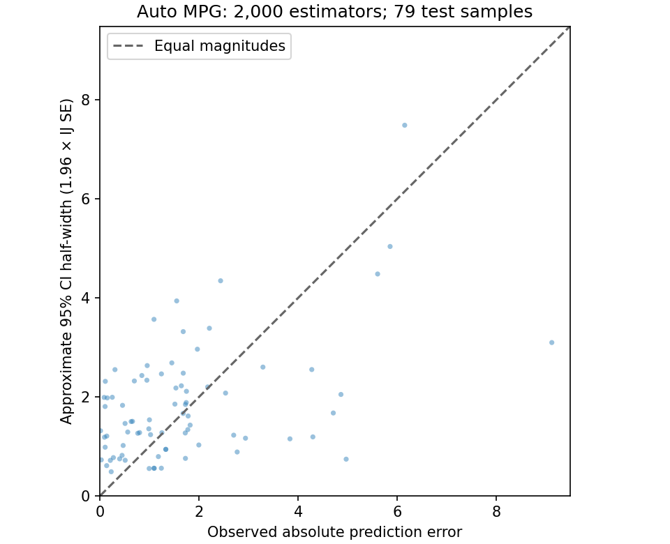
79 held-out samples; 0 negative raw IJ variances clipped to zero for plotting.
California
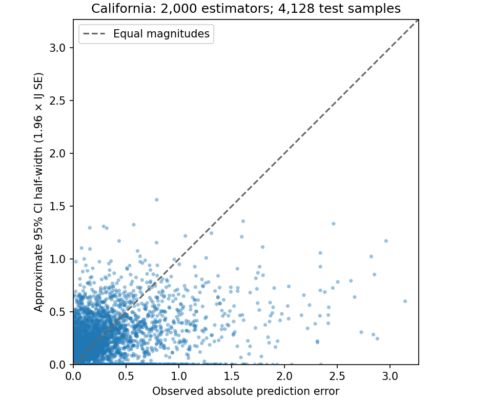
4,128 held-out samples; 1300 negative raw IJ variances clipped to zero for plotting.
Diabetes
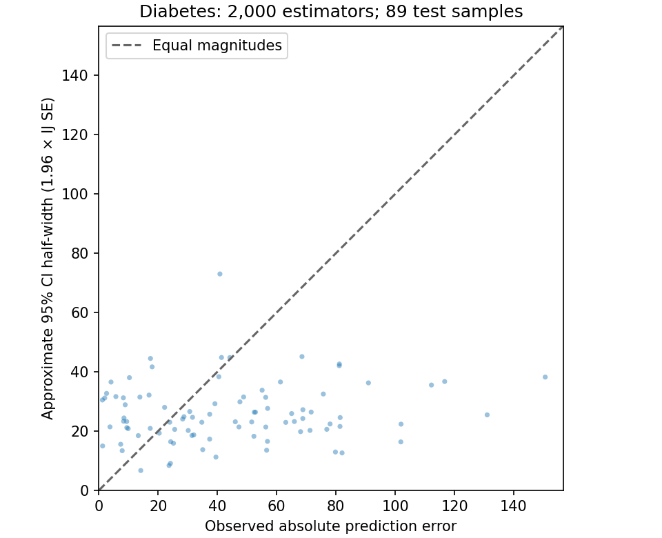
89 held-out samples; 0 negative raw IJ variances clipped to zero for plotting.
Breast Cancer class 1
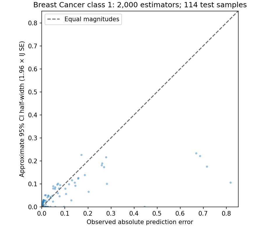
114 held-out samples; 29 negative raw IJ variances clipped to zero for plotting.
Synth Hard class 1
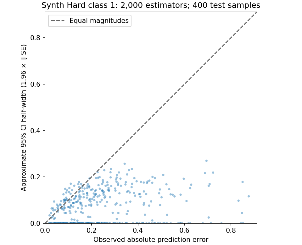
400 held-out samples; 156 negative raw IJ variances clipped to zero for plotting.
Synthetic Reg
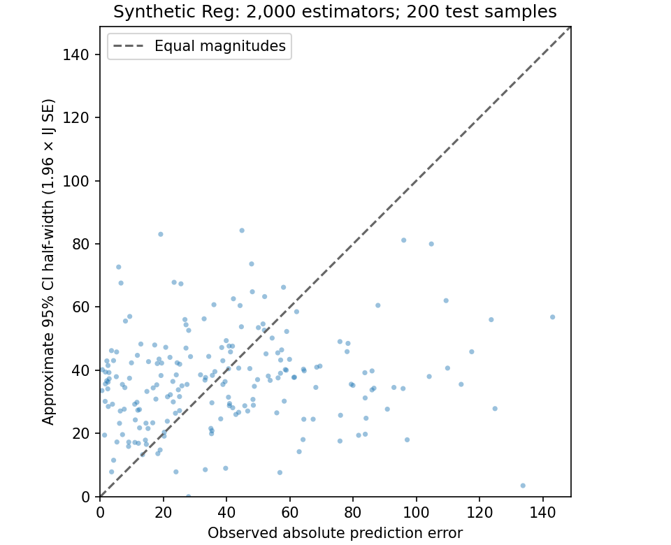
200 held-out samples; 1 negative raw IJ variances clipped to zero for plotting.
Wine class 0
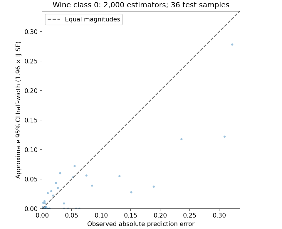
36 held-out samples; 12 negative raw IJ variances clipped to zero for plotting.
Wine class 1
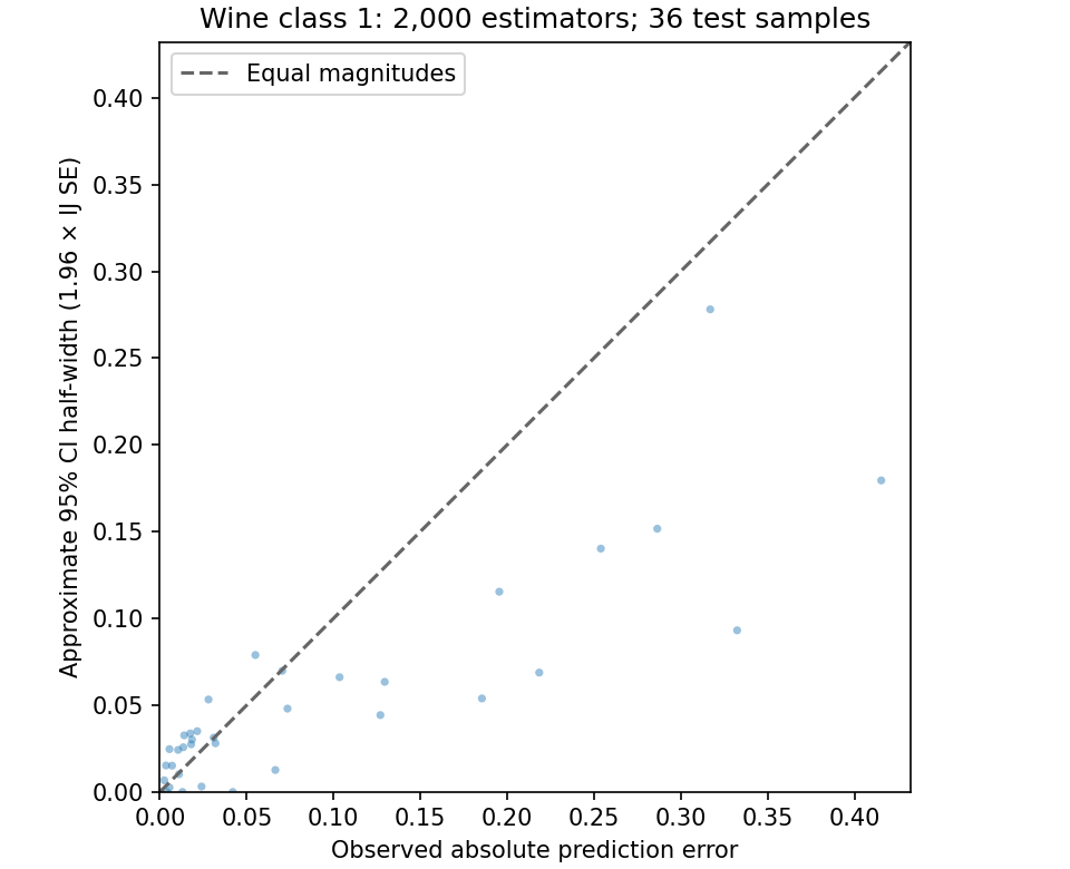
36 held-out samples; 4 negative raw IJ variances clipped to zero for plotting.
Wine class 2
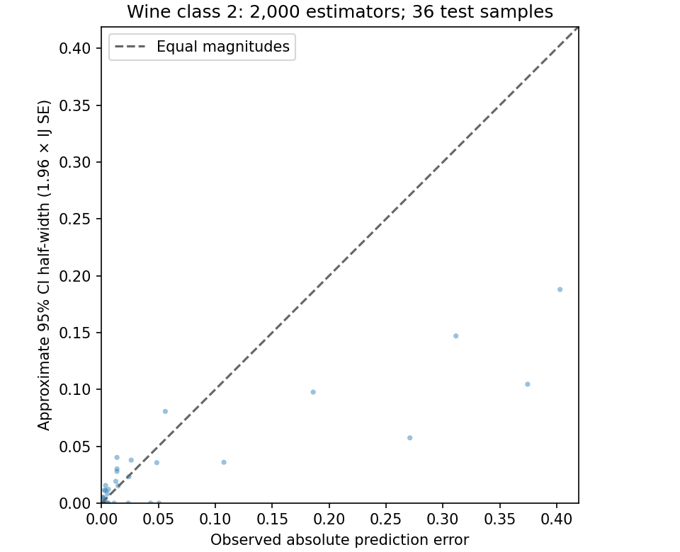
36 held-out samples; 13 negative raw IJ variances clipped to zero for plotting.
Spam
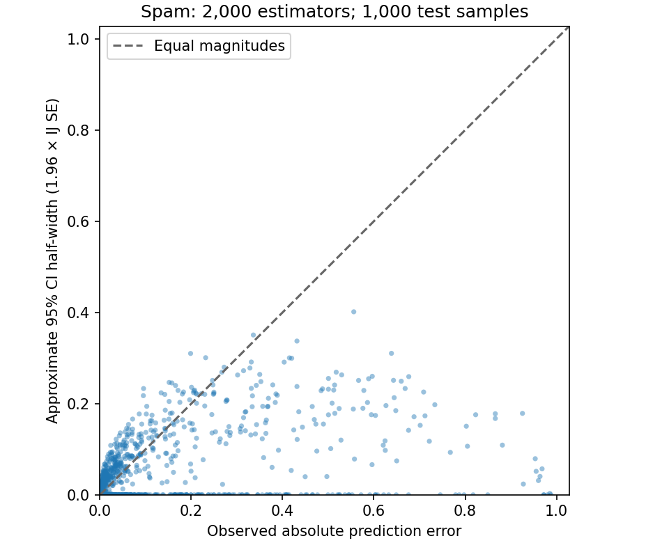
1,000 held-out samples; 422 negative raw IJ variances clipped to zero for plotting.
Auto MPG bagged SVR
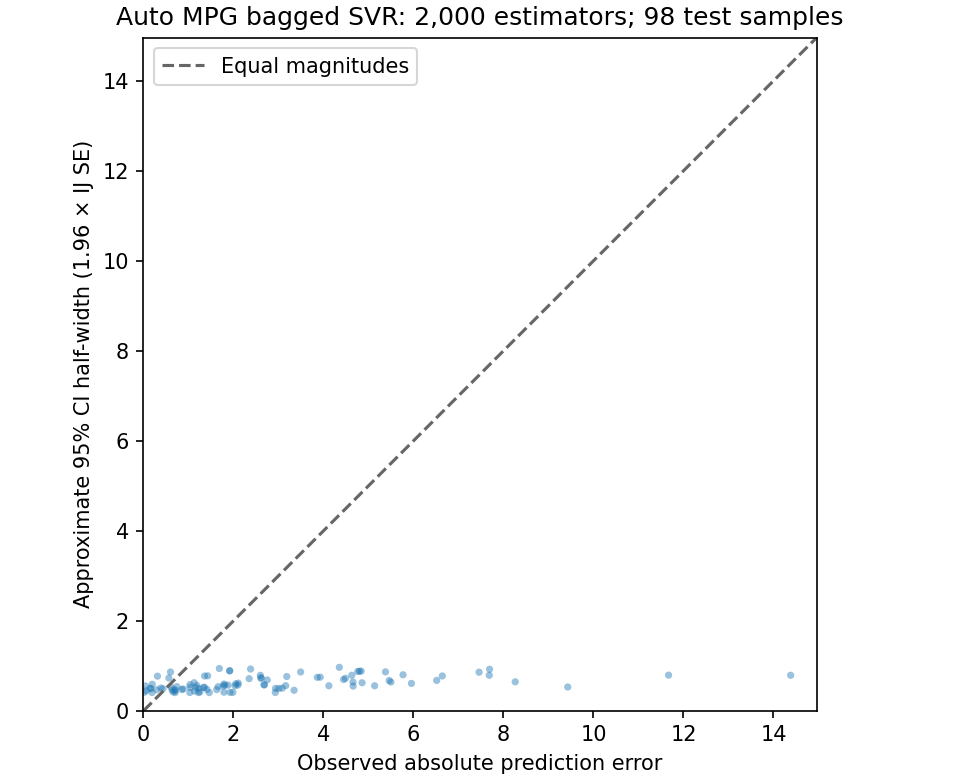
98 held-out samples; 0 negative raw IJ variances clipped to zero for plotting.