Show U-curve of regularization

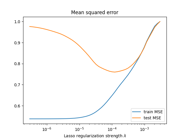
Illustrate the sweet spot of regularization: not too much, not too little. We showcase that for the Lasso estimator on the rcv1.binary dataset.

import numpy as np
from numpy.linalg import norm
import matplotlib.pyplot as plt
from libsvmdata import fetch_libsvm

from sklearn.model_selection import train_test_split
from sklearn.metrics import mean_squared_error

from skglm import Lasso

First, we load the dataset and keep 2000 features. We also retrain 2000 samples in training dataset.

X, y = fetch_libsvm("rcv1.binary")

X = X[:, :2000]
X_train, X_test, y_train, y_test = train_test_split(X, y)
X_train, y_train = X_train[:2000], y_train[:2000]

file_sizes:   0%|                                   | 0.00/13.7M [00:00<?, ?B/s]
file_sizes:   0%|                           | 24.6k/13.7M [00:00<01:48, 126kB/s]
file_sizes:   0%|                           | 49.2k/13.7M [00:00<01:47, 127kB/s]
file_sizes:   1%|▏                           | 106k/13.7M [00:00<01:06, 204kB/s]
file_sizes:   2%|▍                           | 221k/13.7M [00:00<00:37, 356kB/s]
file_sizes:   3%|▉                           | 451k/13.7M [00:00<00:20, 653kB/s]
file_sizes:   7%|█▊                         | 909k/13.7M [00:01<00:10, 1.23MB/s]
file_sizes:  13%|███▍                      | 1.83M/13.7M [00:01<00:05, 2.37MB/s]
file_sizes:  27%|██████▉                   | 3.66M/13.7M [00:01<00:02, 4.59MB/s]
file_sizes:  38%|█████████▉                | 5.23M/13.7M [00:01<00:01, 5.68MB/s]
file_sizes:  57%|██████████████▉           | 7.86M/13.7M [00:01<00:00, 7.97MB/s]
file_sizes:  69%|█████████████████▊        | 9.43M/13.7M [00:02<00:00, 8.05MB/s]
file_sizes:  80%|████████████████████▊     | 11.0M/13.7M [00:02<00:00, 8.13MB/s]
file_sizes:  99%|█████████████████████████▊| 13.6M/13.7M [00:02<00:00, 9.66MB/s]
file_sizes: 100%|██████████████████████████| 13.7M/13.7M [00:02<00:00, 5.41MB/s]

Next, we define the regularization path. For Lasso, it is well know that there is an alpha_max above which the optimal solution is the zero vector.

alpha_max = norm(X_train.T @ y_train, ord=np.inf) / len(y_train)
alphas = alpha_max * np.geomspace(1, 1e-4)

Let’s train the estimator along the regularization path and then compute the MSE on train and test data.

mse_train = []
mse_test = []

clf = Lasso(fit_intercept=False, tol=1e-8, warm_start=True)
for idx, alpha in enumerate(alphas):
    clf.alpha = alpha
    clf.fit(X_train, y_train)

    mse_train.append(mean_squared_error(y_train, clf.predict(X_train)))
    mse_test.append(mean_squared_error(y_test, clf.predict(X_test)))

Finally, we can plot the train and test MSE. Notice the “sweet spot” at around 1e-4, which sits at the boundary between underfitting and overfitting.

plt.close('all')
plt.semilogx(alphas, mse_train, label='train MSE')
plt.semilogx(alphas, mse_test, label='test MSE')
plt.legend()
plt.title("Mean squared error")
plt.xlabel(r"Lasso regularization strength $\lambda$")
plt.show(block=False)