Benchmark of Radius Clustering using multiple datasets and comparison with custom MDS

This example demonstrates how to implement a custom solver for the MDS problem and use it within the Radius Clustering framework. Plus, it compares the results of a naive implementation using the NetworkX library with the Radius Clustering implementation.

The example includes:

1. Defining the custom MDS solver.

2. Defining datasets to test the clustering.

3. Applying Radius clustering on the datasets using the custom MDS solver.

4. Ensure this solution works.

5. Establish a benchmark procedure to compare the Radius clustering with a naive implementation using NetworkX.

6. Comparing the results in terms of :

   • Execution time

   • Number of cluster found

7. Visualizing the benchmark results.

8. Visualizing the clustering results.

This example is useful for understanding how to implement a custom MDS solver and how to perform an advanced usage of the package.

# Author: Haenn Quentin
# SPDX-License-Identifier: MIT

Import necessary libraries

Since this example is a benchmark, we need to import the necessary libraries to perform the benchmark, including NetworkX for the naive implementation, matplotlib for visualization, and sklearn for the datasets.

import networkx as nx
import numpy as np
import matplotlib.pyplot as plt
import time
import warnings

from sklearn.datasets import fetch_openml
from radius_clustering import RadiusClustering
from sklearn.metrics import pairwise_distances_argmin

warnings.filterwarnings("ignore", category=RuntimeWarning, module="sklearn")

Define a custom MDS solver

We define a custom MDS solver that uses the NetworkX library to compute the MDS. Note the signature of the function is identical to the one used in the RadiusClustering class.

def custom_solver(n: int, edges: np.ndarray, nb_edges: int, random_state=None):
    """
    Custom MDS solver using NetworkX to compute the MDS problem.

    Parameters:
    -----------
    n : int
        The number of points in the dataset.
    edges : np.ndarray
        The edges of the graph, flattened into a 1D array.
    nb_edges : int
        The number of edges in the graph.
    random_state : int | None
        The random state to use for reproducibility.

    Returns:
    --------
    centers : list
        A sorted list of the centers of the clusters.
    mds_exec_time : float
        The execution time of the MDS algorithm in seconds.
    """
    G = nx.Graph()
    G.add_edges_from(edges)

    start_time = time.time()
    centers = list(nx.algorithms.dominating.dominating_set(G))
    mds_exec_time = time.time() - start_time

    centers = sorted(centers)

    return centers, mds_exec_time

Define datasets to test the clustering

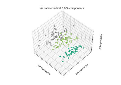
We will use 4 datasets to test the clustering: 1. Iris dataset 2. Wine dataset 3. Breast Cancer dataset (WDBC) 4. Vehicle dataset These are common datasets used in machine learning and lead to pretty fast results. Structure of the variable DATASETS: - The key is the name of the dataset. - The value is a tuple containing:

• The dataset fetched from OpenML.

• The radius to use for the Radius clustering. (determined in literature, see references on home page)

DATASETS = {
    "iris": (fetch_openml(name="iris", version=1, as_frame=False), 1.43),
    "wine": (fetch_openml(name="wine", version=1, as_frame=False), 232.09),
    "glass": (fetch_openml(name="glass", version=1, as_frame=False), 3.94),
    "ionosphere": (fetch_openml(name="ionosphere", version=1, as_frame=False), 5.46),
    "breast_cancer": (fetch_openml(name="wdbc", version=1, as_frame=False), 1197.42),
    "synthetic": (fetch_openml(name="synthetic_control", version=1, as_frame=False), 70.12),
    "vehicle": (fetch_openml(name="vehicle", version=1, as_frame=False), 155.05),
    "yeast": (fetch_openml(name="yeast", version=1, as_frame=False), 0.4235),
}

Define the benchmark procedure

We define a function to perform the benchmark on the datasets. The procedure is as follows: 1. Creates an instance of RadiusClustering for each solver. 2. For each instance, fit the algorithm on each dataset. 3. Store the execution time and the number of clusters found for each dataset. 4. Return the results as a dictionary.

def benchmark_radius_clustering():
    results = {}
    exact = RadiusClustering(manner="exact", radius=1.43)
    approx = RadiusClustering(manner="approx", radius=1.43)
    custom = RadiusClustering(
        manner="custom", radius=1.43
    )
    custom.set_solver(custom_solver) # Set the custom solver
    algorithms = [exact, approx, custom]
    # Loop through each algorithm and dataset
    for algo in algorithms:
        algo_results = {}
        time_algo = []
        clusters_algo = []
        # Loop through each dataset
        for name, (dataset, radius) in DATASETS.items():
            X = dataset.data
            # set the radius for the dataset considered
            setattr(algo, "radius", radius)
            # Fit the algorithm
            t0 = time.time()
            algo.fit(X)
            t_algo = time.time() - t0

            # Store the results
            time_algo.append(t_algo)
            clusters_algo.append(len(algo.centers_))
        algo_results["time"] = time_algo
        algo_results["clusters"] = clusters_algo
        results[algo.manner] = algo_results

    return results

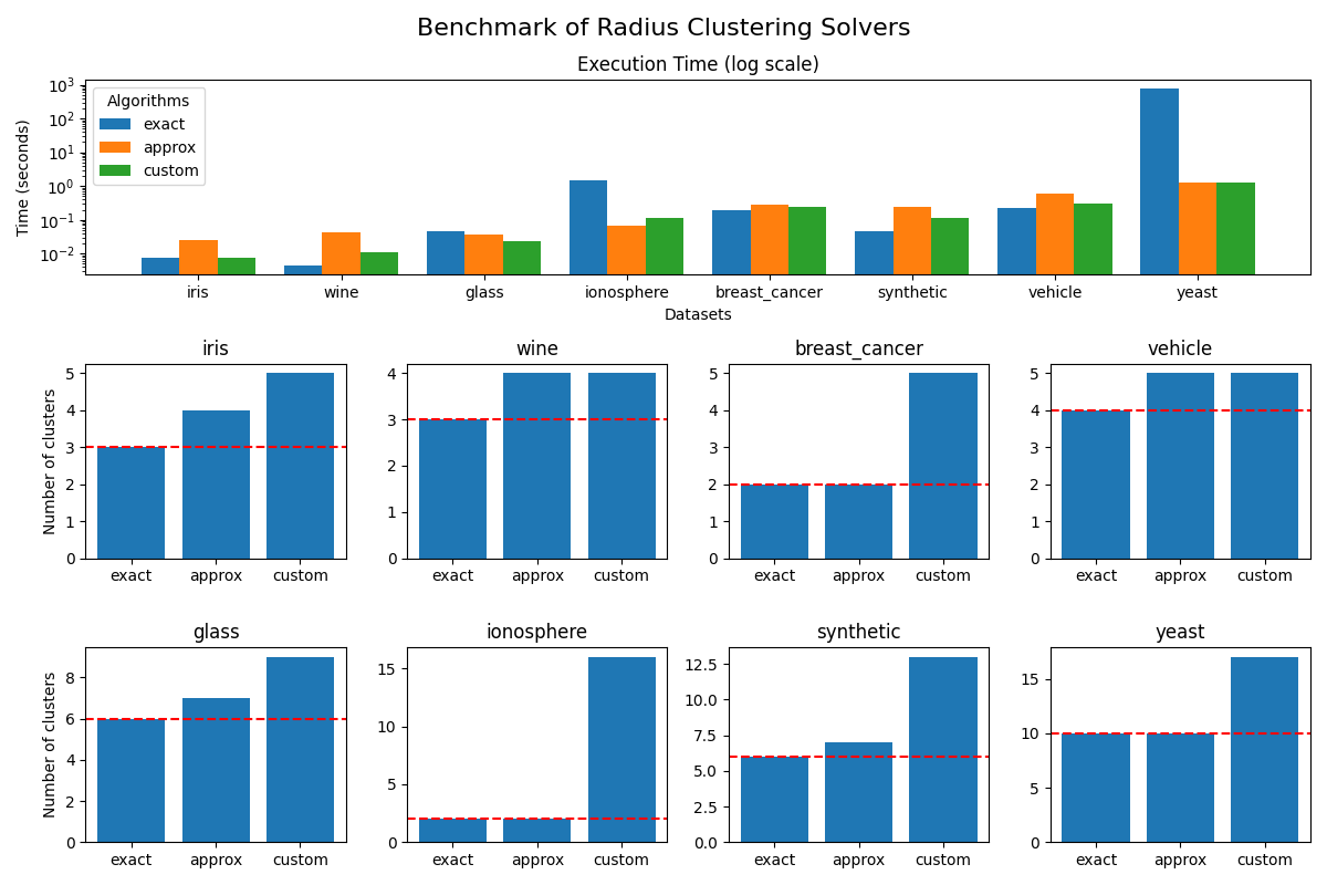
Run the benchmark and plot the results

We run the benchmark and plot the results for each dataset.

results = benchmark_radius_clustering()

# Plot the results
fig, axs = plt.subplot_mosaic(
    [
        ["time", "time", "time", "time"],
        ["iris", "wine", "breast_cancer", "vehicle"],
        ["glass", "ionosphere", "synthetic", "yeast"],
    ],
    layout="constrained",
    figsize=(12, 8),
)
fig.suptitle("Benchmark of Radius Clustering Solvers", fontsize=16)

axs['time'].set_yscale('log')  # Use logarithmic scale for better visibility

algorithms = list(results.keys())
dataset_names = list(DATASETS.keys())
n_algos = len(algorithms)
x_indices = np.arange(len(dataset_names))  # the label locations
bar_width = 0.8 / n_algos  # the width of the bars, with some padding

for i, algo in enumerate(algorithms):
    times = results[algo]["time"]
    # Calculate position for each bar in the group to center them
    position = x_indices - (n_algos * bar_width / 2) + (i * bar_width) + bar_width / 2
    axs['time'].bar(position, times, bar_width, label=algo)

for i, (name, (dataset, _)) in enumerate(DATASETS.items()):
    axs[name].bar(
        results.keys(),
        [results[algo]["clusters"][i] for algo in results.keys()],
        label=name,
    )
    axs[name].axhline(
        y=len(set(dataset.target)),  # Number of unique classes in the dataset
        label="True number of clusters",
        color='r',
        linestyle='--',
    )
    axs[name].set_title(name)

axs["iris"].set_ylabel("Number of clusters")
axs["glass"].set_ylabel("Number of clusters")

axs['time'].set_title("Execution Time (log scale)")
axs['time'].set_xlabel("Datasets")
axs['time'].set_ylabel("Time (seconds)")
axs['time'].set_xticks(x_indices)
axs['time'].set_xticklabels(dataset_names)
axs['time'].legend(title="Algorithms")
plt.tight_layout()
plt.show()

/home/runner/work/radius_clustering/radius_clustering/examples/plot_benchmark_custom.py:223: UserWarning: The figure layout has changed to tight
  plt.tight_layout()

Conclusion

In this example, we applied Radius clustering to the Iris and Wine datasets and compared it with KMeans clustering. We visualized the clustering results and the difference between the two clustering algorithms. We saw that Radius Clustering can lead to smaller clusters than kmeans, which produces much more equilibrate clusters. The difference plot can be very useful to see where the two clustering algorithms differ.

Related examples

Iris Dataset Clustering Example

Iris Dataset Clustering Example